


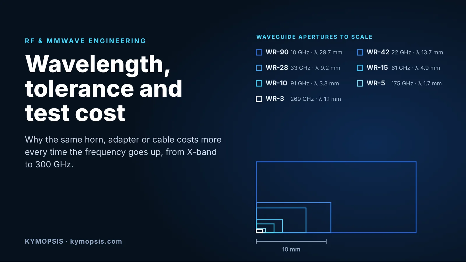
Ask three suppliers to quote the same standard gain horn in X-band and again in WR-10, and the unit price will usually move by much more than the change in material. The waveguide port shrinks from 22.86 mm to 2.54 mm wide, but the drawing tolerances, the surface finish, the flange, the test bench and the scrap rate all move with the wavelength, and each of them moves with the wavelength or faster.
This note puts numbers on that. It covers the wavelength and waveguide size of each band, how much dimensional error a band can absorb, why wall roughness becomes a first-order loss term, and how the measurement setup changes as you go up in frequency. The figures were computed from standard closed-form expressions; the scripts and assumptions are listed at the end so you can rerun them with your own numbers.
Wavelength and waveguide size, band by band
Free-space wavelength is λ0 = c/f: 30 mm at 10 GHz, 5 mm at 60 GHz, 3.9 mm at 77 GHz, 1 mm at 300 GHz. A rectangular waveguide used in its dominant TE10 mode has a broad wall a of roughly 0.7 to 0.8 λ0 at mid-band and a narrow wall b ≈ a/2, so every feature of a waveguide part scales with the wavelength.

| Band | Inside a × b (mm) | TE10 range (GHz) | λ0 at centre (mm) | λg at centre (mm) | Smooth-copper loss (dB/m) |
|---|---|---|---|---|---|
| WR-90 | 22.86 × 10.16 | 8.2–12.4 | 29.7 | 39.1 | 0.11 |
| WR-42 | 10.67 × 4.32 | 18–26.5 | 13.7 | 17.9 | 0.36 |
| WR-28 | 7.11 × 3.56 | 26.5–40 | 9.2 | 12.1 | 0.57 |
| WR-15 | 3.76 × 1.88 | 50–75 | 4.9 | 6.5 | 1.5 |
| WR-12 | 3.10 × 1.55 | 60–90 | 4.1 | 5.4 | 2.0 |
| WR-10 | 2.54 × 1.27 | 75–110 | 3.3 | 4.3 | 2.7 |
| WR-5 | 1.30 × 0.65 | 140–220 | 1.7 | 2.3 | 7.4 |
| WR-3 | 0.86 × 0.43 | 220–330 | 1.1 | 1.5 | 13.4 |
The loss column is the textbook conductor loss for a perfectly smooth copper wall at the geometric band centre. Measured straight sections are typically higher, often by tens of percent, mostly because of surface roughness and plating; we come back to that below.
Coaxial interconnects follow the same rule. The usable upper frequency of a 50 Ω air line is set by the first higher-order mode, TE11, whose cutoff is roughly where the mean circumference π(D+d)/2 equals one wavelength. That is why the connector families are named after the outer conductor diameter and why each one tops out where it does: SMA at 18 GHz (some to 26.5), 3.5 mm at 26.5 GHz, 2.92 mm at 40, 2.4 mm at 50, 1.85 mm at 67, 1.35 mm at 90 and 1.0 mm at 110 GHz. The same first-order formula puts the TE11 cutoff of a 2.92 mm line near 45 GHz and a 1.0 mm line near 133 GHz; support beads and connector geometry pull the rated limit below that.
How much dimensional error a band can absorb
A convenient way to compare bands is to ask what single wall error would produce a given reflection. Take two otherwise identical sections joined with a step in the broad wall (Δa) or the narrow wall (Δb), use the TE10 power–voltage impedance Z ∝ (b/a)·λg/λ0, and solve for the step that reflects 1 % of the incident voltage, which is a 40 dB return loss.

The result is close to a straight line on a log–log plot. A WR-90 section tolerates a broad-wall step of about 270 µm before it reaches 40 dB return loss. WR-28 tolerates about 85 µm, WR-15 about 45 µm, WR-10 about 30 µm, WR-5 about 15 µm and WR-3 about 10 µm. The narrow wall is slightly more sensitive because Z is directly proportional to b.
Two cautions. First, this is a single, isolated step with the junction susceptance ignored, so it is optimistic. A real part stacks several errors: aperture size, aperture position relative to the flange pins, flange flatness, pin-to-hole clearance and, for split-block designs, the offset between the two halves. Each feature gets only a fraction of the total budget. Second, many specifications are tighter than 40 dB. A 45–50 dB return loss requirement for a precision straight section or a matched load leaves even less room.
Length errors matter for anything that depends on phase: power combiners, orthomode transducers, phase-matched arms and array feeds. The phase error from a length error ΔL is 360°·ΔL/λg. A 10 µm length error is 0.09° in WR-90, 0.3° in WR-28, 0.8° in WR-10 and 2.5° in WR-3. A tolerance that was irrelevant at X-band becomes a design parameter above 100 GHz.
| Band | Broad-wall step for RL 40 dB | Narrow-wall step for RL 40 dB | Phase error per 10 µm length |
|---|---|---|---|
| WR-90 | ≈ 270 µm | ≈ 200 µm | 0.09° |
| WR-42 | ≈ 125 µm | ≈ 85 µm | 0.20° |
| WR-28 | ≈ 85 µm | ≈ 70 µm | 0.30° |
| WR-15 | ≈ 45 µm | ≈ 38 µm | 0.56° |
| WR-10 | ≈ 30 µm | ≈ 25 µm | 0.83° |
| WR-5 | ≈ 15 µm | ≈ 13 µm | 1.6° |
| WR-3 | ≈ 10 µm | ≈ 9 µm | 2.5° |
What the machining shop has to deliver
Put the curve next to process capability and the cost steps become visible. General-purpose CNC milling, holding ±20–25 µm without special effort, comfortably covers everything up to K and Ka band. Around WR-15 to WR-10 the budget for each feature falls into the range of precision milling (roughly ±5–10 µm), which means a better machine, temperature control, more careful fixturing and in-process measurement. Above about 150 GHz you are in micromachining territory. Split-block CNC work at sub-millimetre wavelengths is reported at about 2–3 µm from the design values, and below WR-3 many groups move to silicon micromachining or SU-8 processes instead of milling.
Each step down in tolerance also changes inspection. A WR-90 aperture can be checked with pin gauges and calipers. A WR-10 aperture needs an optical or contact coordinate measurement with a resolution well below the tolerance, and a WR-3 split block needs metrology that many machine shops simply do not have. Inspection time and the rejection rate both land in the unit price.
Wall roughness against skin depth
The current in a waveguide wall flows in a layer about one skin depth thick. For copper, δ ≈ 0.66 µm at 10 GHz, 0.27 µm at 60 GHz, 0.21 µm at 100 GHz and 0.12 µm at 300 GHz. When the surface roughness is comparable to δ, the current follows a longer path and conductor loss rises.

The Hammerstad correction, K = 1 + (2/π)·arctan[1.4·(Rq/δ)²], is the simplest way to see the trend. With an RMS roughness of 0.4 µm, a common result from good milling, the factor is about 1.3 at 10 GHz but about 1.9 at 100 GHz. Hammerstad saturates at 2 and is known to under-predict loss at mmWave, so the real penalty can be larger. The point is the ratio Rq/δ: a finish that is “smooth” for X-band is rough for W-band.
This is why high-band parts specify surface finish on the internal walls, use finishing passes with fresh tools, and are often silver or gold plated. Plating adds its own variables: thickness uniformity in narrow slots, adhesion, and the conductivity of the plated layer itself. The cost of a WR-10 straight section is driven far more by these steps than by the amount of metal.
Measurement and test cost
Every part that leaves a supplier with a datasheet has to be measured on something. At low frequencies one vector network analyzer with N or 3.5 mm ports covers a wide range of products. As the band moves up, three things happen at once.
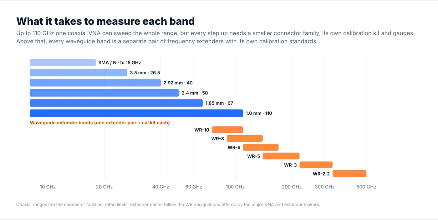
- The connector family changes. Each step from 3.5 mm to 2.92, 2.4, 1.85 and 1.0 mm brings a new set of test cables, adapters, torque wrenches, connector gauges and a calibration kit. Smaller connectors wear faster and need to be gauged more often, and a damaged 1.0 mm interface can take a test port with it.
- Above about 110 GHz each waveguide band is its own setup. The VNA drives a pair of frequency extenders, one per port, each covering a single waveguide band (WR-10, WR-8, WR-6, WR-5, WR-3 and so on), with a calibration kit for that band. A lab that wants to test WR-5 and WR-3 parts needs two extender pairs and two sets of standards.
- The measurement itself gets harder. Flange alignment, cable flexure and thermal drift become a visible fraction of the result, so calibrations are repeated more often and measurement uncertainty has to be stated with the data.
The capital cost of this equipment is spread over the parts that are tested on it. A simple way to see the effect is to write the test cost per unit as
test cost per unit ≈ (C / (Y × H × U)) × t + (calibration and connector care per unit)

C  capital cost of the bench (VNA, extenders, cal kits, cables)
Y  depreciation period in years
H  working hours per year
U  utilisation (share of hours actually spent measuring)
t  hours per unit, including setup and calibration checks
For example, a bench that costs ten times as much, used by a smaller customer base so that utilisation halves, carries twenty times the capital cost per test hour. If the higher-band part also takes longer to mount and verify, the test cost per unit rises faster still. Volumes in the upper bands are small, so this cost is not diluted the way it is for an 18 GHz cable sold in thousands.
This is also why “100 % tested with data” and “sample tested” mean different prices above 40 GHz. When you compare quotes, check which one you are getting.
What this means when you specify or buy
- Tolerance where it matters. Put tight tolerances on the aperture, the flange interface and phase-critical lengths, and relax external features. A blanket ±10 µm on every dimension of a WR-28 part costs money without improving the RF result.
- Specify internal surface finish (Ra or Rq) and plating for anything above about 40 GHz, together with the loss you actually need.
- Flange type. From WR-10 upward, ask whether the flange is a precision UG-387 variant with tighter alignment pins and holes. IEEE 1785.2 standardises such interfaces for 110 GHz and above. Flange mismatch can dominate the return loss of a short part.
- Connector grade and mating. Match connector families instead of adapting across them, torque to the specified value, and gauge connectors before measuring high-band parts.
- Test data. State the frequency points or band, the parameters (S11, S21, gain, pattern), whether each unit is measured, and how the data will be delivered.
Where our catalog parts sit
Our RF & microwave catalog is expanding band by band, with V-band, E-band and higher horns and components on the way. Current parts include:
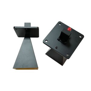
- X-band standard gain horn, 8.2–12.4 GHz, 20 dB and K-band standard gain horn, 17.6–26.7 GHz for antenna range and EMC reference use
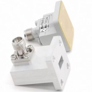
- WR-28 to 2.92 mm waveguide-to-coax adapter, 26.5–40 GHz
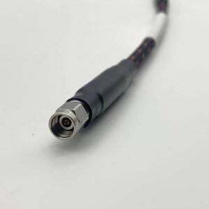
- Armored 2.92 mm test cable, DC–40 GHz, 2.92 mm fixed attenuators and precision adapters
How these parts are actually produced, from split blocks to plated plastic, is covered in machined or metallized plastic. For a band or part that is not listed yet, non-standard apertures, split-block assemblies, or horns and feeds built to a drawing, we quote case by case through our antenna and waveguide machining service. Send the drawing or the electrical target, the band and the quantity, and say whether you need per-unit test data.
Related: radome design for 24–80 GHz radar.
FAQ
What is the wavelength at 60, 77 and 94 GHz?
In free space, 5.0 mm at 60 GHz, 3.9 mm at 77 GHz and 3.2 mm at 94 GHz. Inside a waveguide the guide wavelength λg is longer, for example about 4.1 mm at 94 GHz in WR-10.
What machining tolerance does a WR-10 part need?
As a first-order figure, a single 30 µm step in the broad wall already gives about 40 dB return loss at 90 GHz. Because several errors stack, critical WR-10 features are usually held to around ±5–10 µm, with the flange interface and alignment pins controlled as tightly as the aperture.
Why is a W-band horn so much more expensive than an X-band horn?
The tolerance budget is roughly ten times tighter, surface finish has to be better relative to a skin depth of about 0.2 µm, plating and inspection add steps, and each unit is tested on a waveguide extender setup that serves far fewer parts than a coaxial bench.
Up to what frequency can I use coaxial connectors?
SMA to 18 GHz (some to 26.5), 3.5 mm to 26.5, 2.92 mm to 40, 2.4 mm to 50, 1.85 mm to 67, 1.35 mm to 90 and 1.0 mm to 110 GHz. Above that, waveguide interfaces are the norm.
Does surface roughness matter below 20 GHz?
Less, but not zero. With an RMS roughness of 0.4 µm the Hammerstad factor is already about 1.3 at 10 GHz. For long runs or low-noise front ends it is worth specifying.
How the numbers were computed
Waveguide dimensions and band edges are the standard EIA WR values. Guide wavelength and smooth-wall conductor loss use the TE10 closed-form expressions with copper at σ = 5.8×10⁷ S/m. The tolerance figures use the power–voltage impedance and ignore junction susceptance and higher-order modes, so they are a scaling guide, not a substitute for a tolerance analysis in a full-wave solver. Roughness uses the Hammerstad model. Machining capability ranges are typical values, not guarantees from any particular shop.
Further reading
- IEEE Std 1785.1-2012 and 1785.2-2016, rectangular metallic waveguides and their interfaces for 110 GHz and above.
- IEEE P1785: a new standard for waveguide above 110 GHz, Microwave Journal.
- What’s the difference between coaxial connectors (part 2), Microwaves & RF.
- Coaxial connector handling (1MA99), Rohde & Schwarz application note.
- A 660 GHz CNC-machined waveguide filter, University of Birmingham, including a discussion of CNC accuracy at sub-millimetre wavelengths.
- Millimeter-wave frequency extension for vector network analyzers, Keysight brochure.