



Many radar modules have a single ADC per receive channel and record only real numbers. They still measure micrometre motion, Doppler and angle, and all three are readings of phase. The ADC never recorded a phase. The phase appears in the FFT: every FFT output is a complex number, an I/Q pair, whether the samples going in were real or complex. This post shows how one FFT output is computed, why it has to be complex, and what changes between real and complex (I/Q) sampling. It is the maths behind chapter 2 and chapter 6 of Radar Principles.
What one FFT output computes
Take the beat signal of a radar with one target, sampled N times during a chirp. One FFT output answers one question: how much of a particular frequency is in these samples? To find out, it multiplies every sample by a test tone at that frequency and adds up the products. When the signal contains the test tone, the two rise and fall together, almost every product is positive and the sum is large. When it does not, the products swing both ways and the sum stays near zero.
The figure does this by hand for 64 real samples of a tone that completes exactly 10 cycles, started 40° into its cycle. Multiplying by a cosine that also completes 10 cycles and adding gives 24.5. Multiplying by a negative sine, −sin(2π·10n/64), gives a second sum, 20.6. Those two numbers are the in-phase and quadrature parts, I and Q, of FFT output 10.
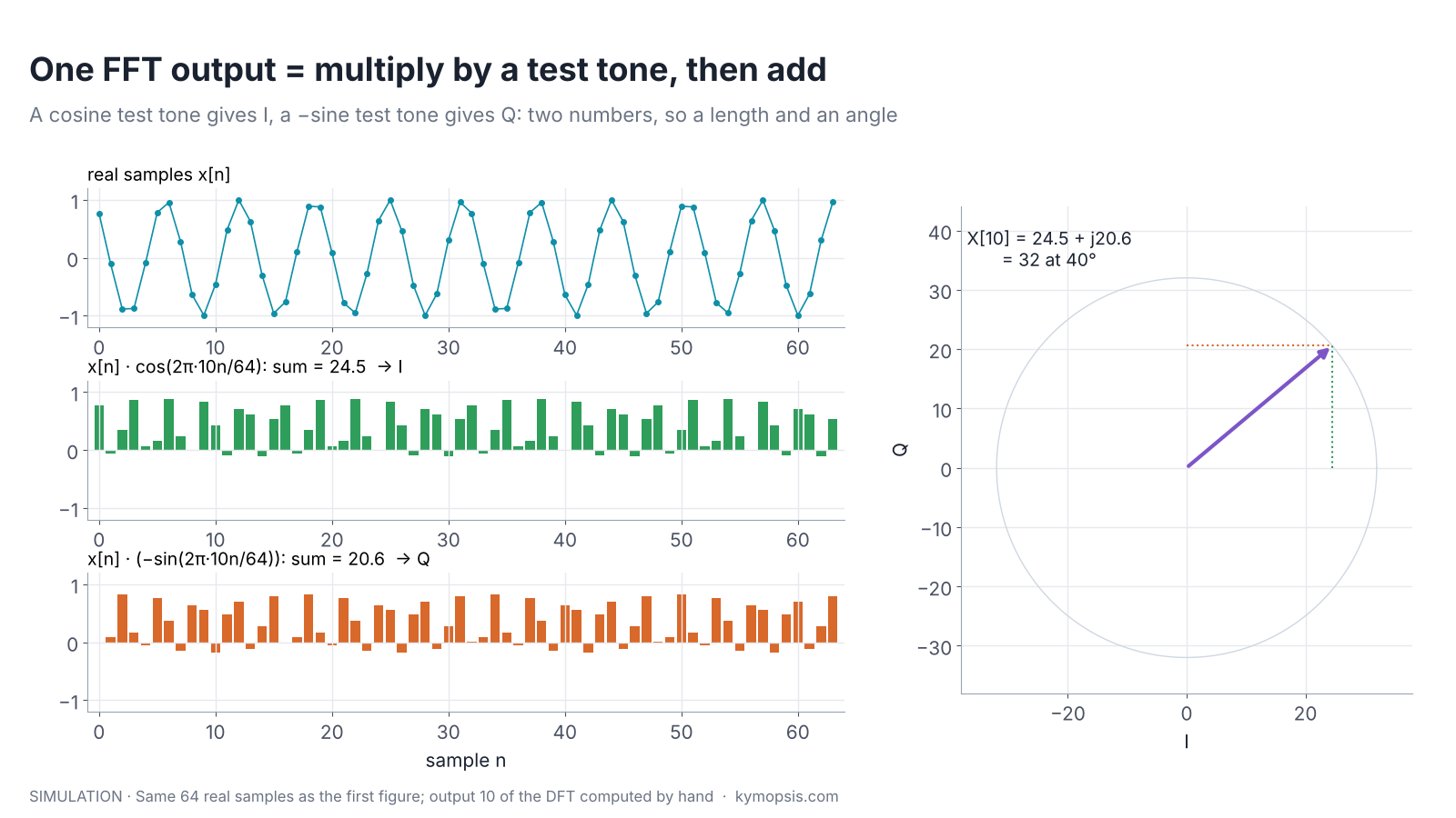
Drawn as an arrow in the I/Q plane, the pair has length √(24.5² + 20.6²) = 32 and angle atan2(20.6, 24.5) = 40°. The angle is exactly the phase the tone started with. Nothing about the samples was complex; the second number came from the second test tone.
The discrete Fourier transform (DFT) repeats this for N test tones, at 0, 1, 2 … N−1 cycles per record, and writes each cosine-and-sine pair as one complex exponential:
X[k] = Σn=0…N−1 x[n] · e−j2πkn/N
Since e−jθ = cos θ − j·sin θ, the real part of each product is the cosine product and the imaginary part is the sine product with a minus sign, which is the bottom row of the figure. The FFT is a fast way to compute all N outputs at once; the numbers are the same.
Why the test tone is complex
A cosine test tone alone would be blind to part of the signal. If the samples are a sine wave, a sine is a cosine shifted by a quarter cycle, and the cosine products sum to zero. The cosine test would report no tone at all. The sine test catches exactly what the cosine test misses, and between them they measure any phase: I = A·cos φ and Q = A·sin φ, the same pair as the two mixers in chapter 2.
That is the reason the DFT uses e−j2πkn/N and not a plain cosine. The complex test tone is two real test tones a quarter cycle apart, and the complex output is a length and an angle. For a radar the length says how strong the echo is and the angle says where, within half a wavelength, the target sits.
Real samples: every tone appears twice
Run the 64 real samples through a full FFT and two peaks appear, at output 10 and at output 54 (64 − 10), each of height 32. With complex samples of the same tone, I and Q from two ADCs, there is one peak of height 64 at output 10 and nothing at 54. The first figure shows both.
The second peak is not a second target. A real cosine is the sum of two arrows of half length that turn in opposite directions:
cos(ωn + φ) = ½·ej(ωn + φ) + ½·e−j(ωn + φ)
One arrow turns forward at +10 cycles per record, the other backward at −10, and the FFT lists −10 as output 54. The two outputs are mirror images, X[54] = X[10]*: same length, opposite phase (+40° and −40° here). For any real input this holds for every pair, X[N−k] = X[k]*, so the upper half of the outputs repeats the lower half and carries nothing new. N real samples give N/2 usable complex outputs; N complex samples give N.
Why X[N−k] is the conjugate of X[k] for real input
For real x[n], take the complex conjugate of the definition: X[k]* = Σ x[n]·e+j2πkn/N. Since ej2πn = 1 for whole n, e+j2πkn/N = e−j2π(N−k)n/N, so the sum is X[N−k]. The amplitude splits evenly between the two outputs, which is why a real tone of amplitude 1 gives N/2 = 32 at each, and a complex tone of amplitude 1 gives N = 64 at one. numpy’s np.fft.rfft uses this and returns only outputs 0 … N/2.
What this means in an FMCW radar
In an FMCW radar the beat frequency of a target is positive and proportional to range (chapter 5). With real sampling the radar keeps outputs 0 to N/2 as range bins and ignores the mirrored half. Each kept bin is a complex number, and its phase is the echo phase 4πR/λ from chapter 2, plus a constant set by the hardware.
The figure tests that with a 60.5 GHz example. A target at 1.5 m moves 3 mm away; at each position the beat signal is sampled once with one ADC and once with two, and the phase of the peak range bin is read. Both lines lie on top of the formula 4πΔR/λ: about 145° per millimetre, one full turn every 2.48 mm.

Everything later chapters build on that phase works the same way with real sampling. Doppler is the bin’s phase turning from chirp to chirp (chapter 10), and angle is the phase difference of the same bin between receive channels (chapter 12). In code the only change is which transform keeps which half:
import numpy as np
# adc: [chirps, samples] for one receive channel
w = np.hanning(adc.shape[-1])
if np.isrealobj(adc):
    rp = np.fft.rfft(adc * w, axis=-1)      # real samples: N/2 + 1 complex bins
else:
    rp = np.fft.fft(adc * w, axis=-1)       # complex samples: N complex bins
phase = np.angle(rp)                        # echo phase per chirp and range bin, either way
Real or complex sampling: what changes
Both schemes are in wide use, and radar chip vendors document both. The choice changes the span of beat frequencies, the hardware count and how the receiver handles anything at a negative frequency. It does not change whether phase, Doppler or angle can be measured.
| Real sampling | Complex (I/Q) sampling | |
|---|---|---|
| ADCs per receive channel | 1 | 2 |
| Usable FFT outputs | N/2 + 1 (from N real numbers; outputs 0 and N/2 are real) | N (from N complex samples = 2N real numbers) |
| Beat frequencies covered at sample rate fs | 0 to fs/2 | −fs/2 to +fs/2, cleanly only down to the image rejection |
| Maximum range at slope S | fs·c / (4S) | up to fs·c / (2S), limited by I/Q balance (see below) |
| Phase, Doppler, angle per bin | yes | yes |
| Tells +f from −f | no, they land on the same bin | yes, to the image rejection (often 25–40 dB, see below) |
| Hardware and data | fewer converters, half the samples | two matched paths; gain and phase mismatch must be calibrated |
The last two rows are the real trade. A real-sampling receiver cannot tell a tone turning forward from one turning backward. For targets that does not matter, because their beat frequencies are all on the positive side. It matters for anything that lands at a negative frequency, such as another radar’s chirp crossing yours or noise from the mixer’s image band. With real sampling, and a single real mixer in front of it, that lands on the same bins as the wanted echoes; a quadrature mixer with complex sampling can keep it apart. Complex sampling keeps them apart, but only as well as the two paths match; an I/Q imbalance creates a small mirror of its own (chapter 2).

A real-sampling design therefore keeps all wanted beat frequencies inside 0 to fs/2 and filters the rest before the ADC (chapter 5). A complex-sampling design can in principle cover twice the span from the same sample rate and reject mirrored interference, and pays with a second converter per channel. How much of that it really gets depends on how well the two paths match, which is the next section.
I/Q balance: how much of the extra span is usable
Complex sampling assumes the Q path is an exact copy of the I path shifted by 90°: same gain, same quarter-turn delay, same filter. Real hardware gets close but not exact. The two mixers, filters and ADCs differ by a fraction of a decibel in gain and by a degree or more in phase, and both errors change with frequency and temperature. With a gain ratio g between the paths and a phase error φ, a tone at +f no longer lands only at +f: part of it appears at −f. The ratio of the wanted tone to that mirror is the image rejection ratio,
IRR = (1 + 2g·cos φ + g²) / (1 − 2g·cos φ + g²), usually quoted in dB.

Worked through: 1 dB of gain error and 5° of phase error give an IRR of 22.8 dB, so every echo leaves a mirror about 23 dB weaker at the opposite frequency. Bringing the paths to 0.1 dB and 1° raises it to 39.6 dB. Even a perfect gain match with 2° of phase error stops at about 35 dB. Those mirrors decide what the negative half of the spectrum is good for.
- Range is not simply doubled. If a radar uses 0 to fs to reach twice the range, the mirror of a strong close target lands at a far range bin as a ghost target, IRR below the real echo. Echo power falls with the fourth power of range, so a target ten times farther is already about 40 dB weaker than one of the same size up close. Far targets weaker than (close echo − IRR) sit under the ghosts, and the extra span is only as usable as the image rejection allows.
- Interference is pushed down, not removed. A strong interferer at −f leaves a residue at +f IRR below its own level. With 30 dB of rejection, an interferer 50 dB above a weak echo still lands 20 dB above it.
- Calibration helps, within limits. Measuring g and φ with a known test tone and correcting the samples digitally typically raises image rejection well beyond the raw hardware figure, but filter mismatch makes the error depend on frequency, so a single correction does not hold across the whole band or over temperature. Chip datasheets state it as I/Q gain and phase mismatch or as image rejection; that is the number to check.
This is why many complex-sampling radars still place their targets on the positive side only and use the negative half for interference detection and noise estimation, rather than counting it as extra range. In the trade table, complex sampling buys separation of +f and −f to the depth of its I/Q balance, not an automatic factor of two. The same mismatch shows up in chapter 2 as the I/Q circle squashed into a tilted ellipse.
Why it is called fast
Computed directly, every one of N outputs needs N multiplications: 4,096 complex multiplies for 64 samples, 65,536 for 256. The fast Fourier transform gets the same N outputs with about (N/2)·log₂N multiplies, 192 for 64 samples and 1,024 for 256, by noticing that the test tones of a long transform are built from the test tones of shorter ones. Those shared values, e−j2πk/N, are called twiddle factors. How the FFT splits the work, and what fixed-point scaling does to phase, is a later Radar Math post. When a radar needs only a few outputs, computing them one at a time can be cheaper still; chapter 21 uses exactly that for the second receive channel.
Where the clean numbers stop
- Tones between outputs. The example tone completes a whole number of cycles. A real target rarely does, so its energy spreads over neighbouring outputs (leakage), the peak drops and the peak bin’s phase gains an offset that depends on where between bins the tone sits. A window reduces the spreading. Phase changes still track motion, as the third figure shows with a Hann window; chapter 8 covers reading between bins.
- Scaling conventions. numpy’s FFT does not divide by N, so a unit tone gives N/2 (real) or N (complex). Other libraries and radar chips scale differently; compare phases freely, compare amplitudes only after checking the scaling.
- The edges of the real spectrum. Near 0 and near fs/2 a real tone and its mirror overlap, so the closest and farthest bins of a real-sampling radar are less clean. High-pass and anti-alias filters keep targets away from those edges (chapter 5).
FAQ
Does a radar need I/Q sampling to measure phase?
No. Phase is read from the complex FFT bins, and an FFT of real samples gives complex bins. Real-sampling radars measure phase, Doppler and angle the same way; they cover half the beat-frequency span and cannot separate a tone from its mirror at a negative frequency.
What is I/Q balance and why does it matter?
It is how closely the Q path matches the I path in gain and in its 90° phase shift. Any mismatch leaves a mirror of each signal at the opposite frequency, so the negative half of a complex spectrum is only clean down to the image rejection ratio. It limits how much extra range or interference rejection complex sampling really delivers.
Why does my FFT of real radar data show two peaks per target?
The second peak is the mirror at output N−k, the complex conjugate of the first. For real input the upper half of the FFT repeats the lower half. Keep outputs 0 to N/2, or use a real-input FFT such as numpy’s rfft.
Is the FFT the same thing as the DFT?
The DFT is the definition, one multiply-and-add per output with a complex test tone. The FFT is an algorithm that computes all DFT outputs with far fewer operations; the results are identical up to rounding.
Which is better for a radar, real or complex sampling?
Neither in general. Complex sampling can cover up to twice the span for a given sample rate and separates negative-frequency interference, but only to the depth of its image rejection (about 23 dB at 1 dB and 5° of I/Q mismatch, about 40 dB at 0.1 dB and 1°); it costs a second ADC per channel and I/Q calibration. Real sampling uses less hardware and data. Both deliver complex range bins with phase.
Sources and method
- A. V. Oppenheim, R. W. Schafer, Discrete-Time Signal Processing, 3rd ed., Pearson, 2010 (DFT, symmetry, FFT).
- R. G. Lyons, Understanding Digital Signal Processing, 3rd ed., Prentice Hall, 2011 (quadrature signals, real vs complex sampling).
- M. A. Richards, Fundamentals of Radar Signal Processing, 2nd ed., McGraw-Hill, 2014 (FMCW range processing).
- NumPy documentation, numpy.fft (scaling and rfft).
- All figures are computed in Python from the formulas shown (ideal tones, no noise; the radar example uses a 58.5–62.5 GHz sweep in 40 µs, 256 samples at 6.4 MS/s and a Hann window). They are simulations, not measurements of a product. Related simulation code is in Kymopsis/radar-basics-sim.