Radar Principles 21: The Real-Time Processing Chain: CFAR, Angle and Tracking

A small 60 GHz radar with 16 virtual channels, 64 chirps and 128 samples per chirp collects 131,072 complex numbers every frame, ten or twenty times a second. A useful output is a short list: two people, where they are and how fast they move. The processing chain is the order of operations that shrinks the first into the second inside the frame time, and its key idea is to decide where the targets are as early as possible and spend the expensive work only there. This chapter puts the pieces of the earlier chapters in that order and shows what each choice costs.

This is chapter 21 of Radar Principles and the one that ties the others together. It uses the range-Doppler map of chapter 10, the CFAR detector and tracker of chapter 16, and the angle methods of chapters 12, 14 and 17.

What has to happen in every frame

A kitchen during dinner service turns a delivery of raw ingredients into a few plates, every evening, in a fixed order: wash, chop, cook, plate. A radar does the same every frame: a flood of raw samples goes in, and a short list of people and their speeds comes out, before the next frame arrives.

Think of a radar frame as a parcel sorting line. Raw samples arrive by the truckload, every parcel has to be looked at once, but only a few contain anything worth opening. The line is fast where it must touch everything and careful only where something was found.

For an FMCW radar the line has seven stations. The range FFT turns each chirp’s samples into a range profile. The Doppler FFT, taken across chirps for every range bin, adds velocity. The power of all channels is added cell by cell into one range-Doppler map. CFAR decides which cells hold a target. Angle is computed for those cells. Points that belong to one object are grouped, and a tracker follows the objects from frame to frame.

The first four stations touch every sample and run on regular, data-independent loops, which is why radar chips and FPGAs implement them in hardware. Everything after CFAR works on a list whose length depends on the scene, which suits a processor. The bar chart shows the reason for the order: an angle FFT over every range-Doppler cell (the so-called 3D FFT) would cost 1.57 million complex multiplies per frame, more than the range and Doppler FFTs combined, to find angles for cells that are almost all empty.

The frame time sets the budget. At 10 frames per second everything above must finish in 100 ms, and in practice much less, because the chirps of the next frame are already arriving. Memory is the other limit: the Doppler FFT needs every chirp of a frame stored before it can start, so the whole cube, or at least its range-FFT output, must sit in RAM. That storage step is called the corner turn, and on small devices it is often the largest single block of memory.

Detect first: CFAR right after the 2-D FFT

A mail room throws away the junk before anyone reads the post. A radar finds the few cells that hold something right after the range and speed maps, and from then on works only on that short list.

Detection belongs immediately after the range-Doppler map, before angle, because it removes about 99.9 % of the data. The map it works on is the non-coherent sum of all channels, |X|² added over the 16 virtual channels. Adding power keeps the full integration gain of the channels for detection without having to know the target’s angle yet.

The detector itself is the CA-CFAR of chapter 16, now with a window in two dimensions: a few guard cells around the cell under test in range and in Doppler, training cells around them, and a threshold of α times the training mean, with α chosen for the wanted false-alarm probability. Two details differ from the one-dimensional case:

• Doppler wraps, range does not. The Doppler axis is circular (a target at the top velocity bin is a neighbour of the bottom bin, see chapter 15), so the window wraps around it. Range has real edges, so near them the window uses only the cells that exist.
• One target lights several cells. Window sidelobes and a target’s own spread put it into neighbouring range and Doppler cells. Keeping only CFAR hits that are local maxima of their 3 × 3 neighbourhood reduces each target to one or two points before angle is computed.

Hardware implementations compute the training sums with running sums along range and Doppler, so the cost per cell is a few additions whatever the window size. Many radar chips and FPGA designs run CFAR in hardware next to the FFTs and hand the processor only a list of hits, often as a bitmap or a table of cell indices with their power and threshold.

Window sizes and the threshold factor in the example

The example uses 2 guard and 4 training cells on each side in Doppler and 2 guard and 8 training cells on each side in range. The training region is the 13 × 21 box minus the 5 × 5 guard box, N = 248 cells, and α = N(P_fa^−1/N − 1) = 14.2 (11.5 dB) for P_fa = 10⁻⁶, very close to the known-noise value of 13.8 because N is large. On 8,192 cells per frame at 10 frames per second that is about one false alarm every 12 seconds, which the tracker’s confirmation rule then removes. Box sums are computed with two cumulative sums, so the cost does not depend on N.

A second channel without its own Doppler FFT

To know one total on a till receipt, you do not need to add up every receipt in the shop, only the lines on that one. A second receive channel needs only one value at each detected cell, and that one value can be added up directly.

Suppose the hardware has room for one full range-Doppler chain but a second receive channel is needed for angle. The second channel still has to deliver a complex value at each detected cell, with the same integration gain and the same phase reference as the first. It does not need a whole Doppler FFT for that: the cells come from the CFAR detector of chapter 16, so the second channel is only needed where that detector found something.

A Doppler FFT output bin is a sum over the chirps of the range-FFT values at one range bin, each multiplied by a known rotation. So the value at one detected cell (range bin r, Doppler bin d) can be computed directly from the stored range-FFT output of that channel:

z(r, d) = Σ_m w[m] · X[m, r] · e^{−j2π·m·(d − M/2)/M}

with M chirps, w the Doppler window and d counted after the FFT shift. This is the same number the full 2-D FFT would give at that cell, not an approximation; in the simulation the two agree to 10⁻¹⁵. It costs M complex multiplies per detection, 64 here, so 30 detections cost about 1,900 multiplies instead of the 24,576 of a full Doppler FFT for that channel, and the second channel needs no corner-turn memory of its own.

Computing the first channel’s value at the cell the same way, rather than reading it from the hardware FFT, keeps both channels through identical arithmetic. That matters when the hardware FFT uses block floating point or scaling that could shift its phase relative to the software path. The same idea, a single-bin DFT or the Goertzel algorithm, appears whenever only a few frequency bins of a long transform are needed.

Angle only where something was found

A night watchman shines his torch only where he heard a noise, not over every wall all night. The radar works out direction only at the cells where it found something.

At each detection the channels hold one complex value each, the snapshot. Its phase steps across the array by 2π·d·sin θ/λ per element (chapter 12), and three digital ways of reading θ from it cover most radars:

• FFT over the channels for every cell. Zero-padded to 64 points this gives an angle spectrum for each range-Doppler cell. Simple and regular, but most of the work lands on empty cells, and the angle is quantised to the FFT grid unless it is interpolated.
• DFT at the detections. The same beam scan (Bartlett beamformer), but only for the detected cells and on any angle grid you choose, uniform in angle rather than in sin θ. Cost: channels × grid points per detection.
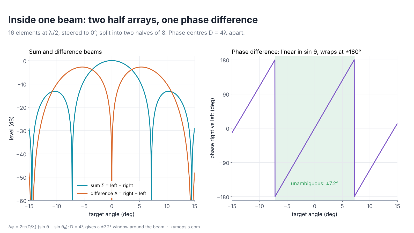
• Coarse subarray DFT, then phase comparison. A DFT over the first few channels on a coarse grid finds roughly where the target is. Two half-array beams are then steered to that coarse angle, and the phase between them gives the fine offset. Cost: a few dozen multiplies per detection.

In a TDM-MIMO radar, where transmitters take turns, one step comes first: a moving target has moved a little between the transmit slots, which adds a Doppler-dependent phase to the channels of the later transmitters. It is removed using the detection’s Doppler bin before any angle method, as explained with the folding problem in chapter 15.

The accuracy panel shows the trade honestly. The 64-point FFT is limited by its grid at about 0.6° RMS no matter how strong the target. The DFT scan follows the noise down to its grid limit. Phase comparison is continuous, so at high SNR it is the most precise of all, but at low SNR the coarse 4-channel stage sometimes picks the wrong neighbourhood and the error jumps. That is acceptable in practice, because a detection at P_fa = 10⁻⁶ usually has 15–20 dB per channel or more after range and Doppler integration, and it is why many designs keep a fallback DFT for weak detections.

Why the half-array phase reads the angle

Split an N-element λ/2 array into a left and a right half and steer both to θ₀ with the same weights. Each half output is a beam with the same shape; the only difference is the position of its phase centre, D = (N/2)·d apart. A target at θ therefore reaches the right half with an extra phase Δφ = 2π·(D/λ)·(sin θ − sin θ₀). Solving, sin θ = sin θ₀ + Δφ·λ/(2πD). The phase wraps at ±π, so the coarse angle must already be within ±asin(λ/2D) of the truth: ±7.2° for D = 4λ, ±3° for D ≈ 9.6λ. (D is the baseline between the two phase centres, not the sweep bandwidth B.) A longer baseline gives finer angle per degree of phase noise but a narrower window, which is the same trade as element spacing against grating lobes in chapter 12.

Three hardware architectures for angle

There are three ways to watch a stage: a camera that records the whole stage at once, a spotlight that follows one actor at a time, or a spotlight with two eyes behind it that also judges where inside the beam the actor stands. MIMO, phased arrays and hybrid monopulse map onto these three.

Where the angle is computed depends on what sits between the antenna elements and the analogue-to-digital converters. Three families cover nearly every radar:

• MIMO, all digital (chapter 14). Every virtual channel reaches the ADC and the angle is computed in software, over the whole field of view in every frame. This is how almost every automotive and industrial radar chip works. The cost is ADC channels, memory and the processing above.
• Phased array, AESA or analog beam (chapter 17). Each element has a phase shifter (and in an active array its own amplifier), and the elements are combined into one output before the ADC. The array forms one narrow, high-gain beam and steers it electronically from one position to the next. The angle comes from which beam position saw the target, refined if needed, and the scene is covered in time rather than in one snapshot.
• Hybrid: analog subarrays plus phase comparison. The array is split into two or more subarrays, each combined in analogue with its own phase shifters and digitised separately. The beam is steered as in a phased array, and inside each beam the phase between the subarray outputs gives the fine angle, exactly as in the previous section. This is the phase-comparison form of monopulse, the technique tracking radars have used for decades to get a fine angle from a single look.

	MIMO (digital)	Phased array (analog beam)	Hybrid subarrays
Channels digitised	all virtual channels	one	two or a few
Field of view per frame	whole	one beam	one beam, fine angle inside it
Angle processing	FFT/DFT, super-resolution	beam index	beam index + phase comparison
Gain per look	one element pattern, integrated digitally	full array gain in the beam	full array gain in the beam
Main costs	ADCs, memory, compute	phase shifters, calibration, scan time	phase shifters, calibration, scan time
Typical use	automotive, industrial, presence	long range, narrow field of view	long range with accurate angle

The simulation in the previous section includes the analog-beam variant: a 16-element array scanned in 5° beam steps, with only the two half-array sums digitised. Its accuracy curve sits on top of the digital phase comparison, because inside a beam it is the same measurement; it needs fewer ADCs, but the beams are visited one after another, and that scan time is paid in update rate.

Two practical limits apply to every architecture that combines in analogue. The phase shifters and the channel paths must be calibrated, because a residual phase error between the two subarrays reads directly as an angle offset (the same effect as an uneven radome in chapter 13). And the step between beam positions has to be smaller than the unambiguous window of the phase comparison, or a target between two beams can be placed in the wrong one.

From detections to tracks in real time

A football commentator calls each player by name as they move, even when two run past each other. A tracker keeps each person’s identity from frame to frame, and has to decide carefully when two paths cross.

The last two stations are the ones of chapter 16, now fed by the chain. Each detection becomes a point with range, velocity and angle, converted to x and y. Points close together in position and velocity are grouped into one object (DBSCAN is a common choice), and the tracker predicts each object forward, gates the new points, associates them and updates a Kalman filter.

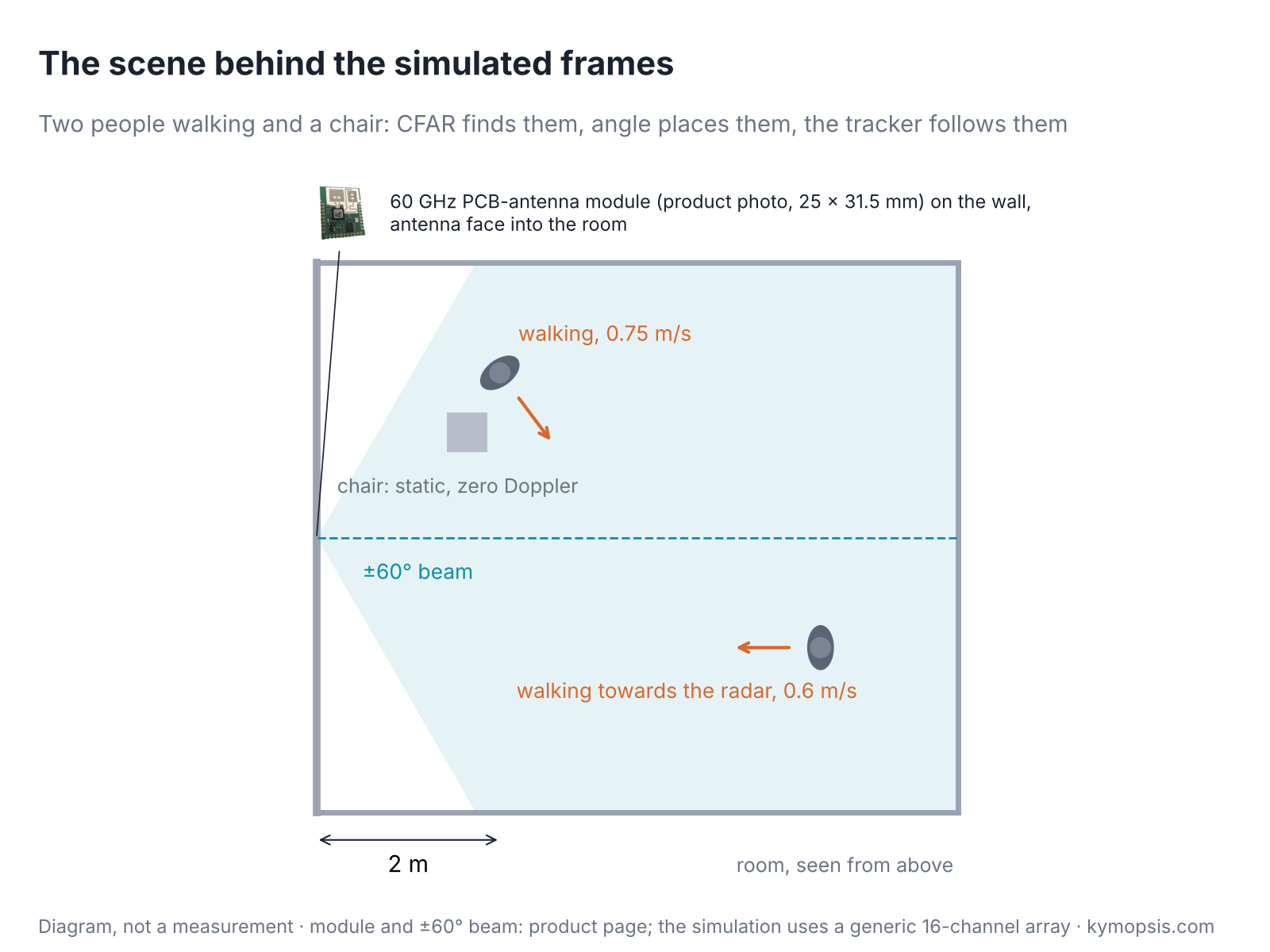
Two choices matter in a real-time system. Association has to be global when tracks are close, because giving each track its nearest point in turn can steal a point from a neighbour; the simple fix used in the example sorts all track-to-detection distances and assigns the smallest first (global nearest neighbour). And zero-Doppler points need a policy: a person walking across the radar’s line of sight has almost no radial velocity for a moment, so dropping all zero-Doppler cells as static clutter makes the track coast through that moment on its prediction. In the simulation the tracks stay locked through it, and the tracked position is about twice as precise as a single detection (1.2 cm against 2.3 cm RMS, mainly range-bin quantisation).

A worked example: a receive-only phased-array module

A recipe from one restaurant kitchen shows how dishes are put together, even though its quantities only fit that kitchen. This module’s numbers belong to it alone, but its structure carries over.

The same choices show up very concretely in an engineering project we worked on: a 77 GHz phased-array module, not a product we sell, with one detail that makes it a good illustration. Each of its two receive chips combines 16 elements through per-element phase shifters into one output, so the module has two analog subarrays and only two IF channels to digitise. It is neither MIMO nor a full AESA, and its numbers do not generalise to other radars; its structure does.

• Beam scan plus phase comparison. The beam is stepped across the field of view in 2.5° positions. Within a beam, the phase between the two subarray outputs gives the offset, and the reported angle is the beam position plus that offset.
• Window matched to the step. The two subarray phase centres are 16 element spacings apart, about 9.6 λ, so one phase comparison covers only about ±3°. That fits the 2.5° beam step; a coarser step would put targets into the wrong beam.
• One full chain, one partial. The FPGA runs range FFT, Doppler FFT and CA-CFAR on the main channel. A second corner-turn memory would not fit, so the second channel stops after the range FFT, and the processor computes both channels’ values at each detection with the single-cell DFT above before comparing their phase.
• Calibration as a parameter. The fixed phase difference between the two channels and the sign convention of the angle are run-time parameters, set with a corner reflector, because they change from board to board.

The open-source ch21_processing_chain.py reproduces this structure with textbook parameters, so the trade-offs above can be explored without the hardware.

Try it yourself: examples/ch21_processing_chain.py in the open-source radar-basics-sim repository runs the whole chain; the building blocks (2-D CFAR, single-cell DFT, the angle methods and the tracker) are in radar_sim/pipeline.py. Change the SNR, the beam step or the CFAR window and see what moves.

What this means on the modules we sell

Buying a ready meal means the kitchen has already done all of this. Our 60 GHz modules run the chain in their firmware and hand you the plates: a list of targets.

The 60 GHz AiP and PCB-antenna development kits are small MIMO radars whose module firmware runs this chain internally and reports detections or targets over a serial link. The module maker does not publish the internal parameters, so the chapter’s numbers are not theirs, but the order of operations explains the behaviour you see: targets appear only after CFAR has found them, angles are least reliable for weak or very close targets, and tracked output lags a fast movement slightly while rejecting single false alarms.

GitHub · Kymopsis /radar-basics-simView repository → B2B engineering · KymopsisDesigning a radar processing chain?Tell us the scene, update rate and the processor or FPGA you plan to use. We scope radar modules and processing for B2B projects.Describe your project

FAQ

Why is CFAR done right after the range-Doppler FFT?

Because it removes almost all of the data. After CFAR only a handful of cells remain, so angle estimation, clustering and tracking run on a short list instead of on every range-Doppler cell.

What is a 3D FFT in radar?

An FFT along the channel (antenna) axis for every range-Doppler cell, giving an angle spectrum everywhere. It is regular and easy to pipeline but spends most of its work on empty cells; computing angle only at detections is far cheaper.

What is monopulse or phase-comparison angle measurement?

Two subarrays (or two antennas) look at the same target; the phase difference between their outputs is proportional to the target’s offset from the beam direction. It gives a fine angle from a single measurement, inside a window of about ±asin(λ/2D) for phase centres D apart.

Is MIMO or a phased array better for measuring angle?

Neither in general. MIMO sees the whole field of view every frame with simple RF and more digital processing; a phased array concentrates gain in one steered beam with fewer ADCs but must scan. Hybrids combine analog subarrays with digital phase comparison.

Sources and method

• M. A. Richards, Fundamentals of Radar Signal Processing, 2nd ed., McGraw-Hill, 2014: range-Doppler processing, CFAR and the processing chain.
• S. M. Sherman, D. K. Barton, Monopulse Principles and Techniques, 2nd ed., Artech House, 2011: amplitude and phase-comparison monopulse.
• R. J. Mailloux, Phased Array Antenna Handbook, 3rd ed., Artech House, 2017: subarrays and analog beam steering.
• Y. Bar-Shalom, X. R. Li, T. Kirubarajan, Estimation with Applications to Tracking and Navigation, Wiley, 2001: gating, association and Kalman tracking.
• Texas Instruments, mmWave SDK / Radar Toolbox documentation, public processing-chain descriptions (ti.com), cited for the common range-Doppler-CFAR-angle order; nothing reproduced.

All figures are computed or simulated with the open-source radar-basics-sim scripts (ch21_processing_chain.py): ideal point targets, white noise, a 2T8R TDM-MIMO array at 60.5 GHz. The worked-example module is described at architecture level only; no measured data from it is shown.