Radar Principles 14: MIMO Radar and the Virtual Array

A radar with two transmitters and four receivers has six antennas, yet its angle processing sees eight receive channels laid out on a gap-free line with twice the aperture of the real receiver row. Three transmitters and four receivers give twelve. That is MIMO radar: each transmitter–receiver pair acts as one virtual receiver at the sum of the two antenna positions, so N_TX × N_RX channels come out of N_TX + N_RX antennas. The catch is that the receivers must be able to tell the transmitters apart, and every way of doing that costs something.

This is chapter 14 of Radar Principles. The angle chapter showed that angle resolution is about 2/N radians for N channels λ/2 apart, so a two-receiver module resolves only about 57°. More receivers cost silicon, pins and board area. MIMO is how radar chips get more channels without that cost.

Why TX + RX positions add

Look closely at many radar chips and you find a small crowd of antennas, for example three that send and four that listen. When the second transmitter takes its turn it sits a little further along, so to the four receivers the whole scene looks shifted, as if they had moved four places along; the third transmitter does the same again. Three times four makes twelve receivers in a row, and the direction sharpens from about 29° to under 10°, without twelve real receive chains.

An echo’s phase records the whole trip: from the transmit antenna to the target and back to the receive antenna. Chapter 12 measured angle by moving the receive end: two receivers a distance d apart see paths that differ by d·sin θ. Nothing in that argument cares which end of the trip moves. Shift the transmitter by d instead and the outgoing leg changes by the same d·sin θ, so the echo phase changes by the same amount.

So two transmitters and one receiver behave like one transmitter and two receivers, as long as the radar can tell which transmitter each echo came from. With two transmitters and four receivers, every transmitter-receiver pair is one channel, eight in all, each behaving like a receiver at the sum of the two antenna positions. That imaginary array of eight is the virtual array. In positions, the rule is exact:

Follow one path. The transmitter at position x_T sends a chirp; a far-field target at angle θ reflects it; a receiver at x_R picks it up. Relative to an antenna at the origin, the outbound leg is shorter by x_T·sin θ and the return leg by x_R·sin θ, so the echo’s phase carries 2π(x_T + x_R)·sin θ/λ. That is exactly the phase that a single receiver at x_T + x_R would see with a transmitter at the origin.

So the set of virtual elements is every TX position added to every RX position, a spatial convolution of the two arrays. Choose the transmitter spacing equal to the full length of the receiver row, N_RX·λ/2, and the copies sit end to end: 2T4R gives a filled line of eight elements spanning 3.5λ, the aperture of an eight-receiver radar. Space the transmitters closer and some virtual elements overlap (2T4R with the TX λ apart gives only six distinct positions); space them wider and gaps appear, which is the starting point for sparse arrays and the grating-lobe problems discussed in the ambiguity chapter.

Elevation works the same way in two dimensions. Raise one transmitter by λ/2 and its four virtual channels land on a second row, half a wavelength above the others. This 3T4R arrangement, eight azimuth elements plus four raised ones, is a common layout on 77 GHz evaluation boards: fine azimuth, coarse elevation, from seven antennas.

Telling the transmitters apart

Two friends calling you on one line at the same time sound like a jumble. They can take turns, one sentence each, or both keep talking while each uses a pattern you know, so you can sort the voices out afterwards. Radar transmitters share one band, and they are told apart in the same two ways: taking turns, or each wearing its own pattern from chirp to chirp.

The virtual-array argument works only if each receiver can separate the echo of TX1 from the echo of TX2. Both transmitters sweep the same band, so they cannot simply be filtered apart. Radar chips use three families of schemes, all of which work across chirps:

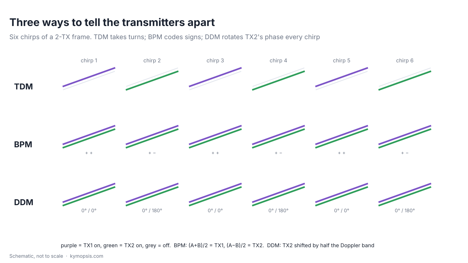
TDM: take turns

Time-division multiplexing is the simplest: chirp 1 from TX1, chirp 2 from TX2, and so on. Each received chirp belongs to exactly one transmitter. It is the default mode on many single-chip radars because nothing has to be decoded. Its costs are covered below: each transmitter repeats only every N_TX chirps, and the target moves between the slots.

BPM: all on, with sign codes

Binary phase modulation switches every transmitter on for every chirp and flips the sign of some of them. With two transmitters, chirp A sends TX1 + TX2 and chirp B sends TX1 − TX2; adding and subtracting the two received chirps recovers each transmitter’s echo. With more transmitters the sign patterns are rows of a Hadamard matrix. Because every transmitter radiates all the time, the frame collects N_TX times more energy than TDM, about 3 dB for two transmitters, if each transmitter runs at full power; under a total EIRP limit the gain can shrink. The decoding assumes the target does not move between the coded chirps, so it has its own motion error.

DDM: all on, separated in Doppler

Doppler-division multiplexing also keeps every transmitter on, but adds a different phase step per chirp to each one. A phase that advances by a fixed amount every chirp looks, after the Doppler FFT, exactly like a Doppler shift. Give TX2 an extra 180° per chirp and its copy of every target moves by half the Doppler band.

DDM keeps the full SNR of simultaneous transmission and has no motion error between slots, which is why DDM is increasingly used in newer automotive radars. The cost is that the Doppler band is shared: with N_TX transmitters each gets 1/N_TX of it, and a fast target from one transmitter can land in another’s slot. Practical DDM schemes leave some slots empty so the processing can tell which copy is which.

The price of TDM

Two photographers sharing one camera each get only every other photo. With time-division, each transmitter fires only on its own turn, so it samples a moving target less often, and a target that moves between the turns looks slightly shifted in angle.

Less unambiguous velocity

With TDM, the time between two chirps of the same transmitter grows by N_TX. The Doppler phase is sampled once per that interval, and the maximum unambiguous velocity is λ/(4·T_repeat). In our simulated 60.5 GHz radar with 50 µs per chirp, one transmitter gives ±24.8 m/s, two give ±12.4 m/s and three ±8.3 m/s. Indoors that rarely matters; on a road it does, and faster targets fold over to wrong velocities. How radars unfold them is in the ambiguity chapter.

The target moves between slots

TX2’s chirp happens one chirp period after TX1’s. A target moving at radial speed v has travelled v·T_c in between, which adds 4π·v·T_c/λ of phase to all of TX2’s virtual channels. The angle processing cannot tell this phase from an angle, so the estimate is biased and the sidelobes rise.

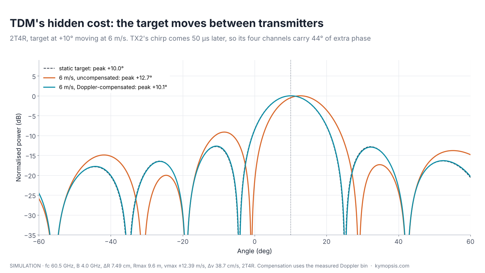
The fix is to use the Doppler that the radar has just measured. The Doppler FFT gives the phase advance per TX repeat interval; dividing it by N_TX gives the advance per slot, and each transmitter’s channels are rotated back by its slot number times that amount before the angle FFT. In our simulation the bias drops from 0.45° at 1 m/s and 2.70° at 6 m/s to 0.05–0.10°, the residual coming from the Doppler bin size. The compensation is only as good as the velocity estimate: if the velocity has folded, the correction is wrong too, which is why velocity unfolding and angle estimation are often solved together.

The compensation, step by step

Let the Doppler peak be at bin k of an M-point Doppler FFT, centred so that bins run from −M/2 to M/2−1. The phase advance between successive chirps of the same transmitter is Δψ = 2πk/M. With N_TX transmitters taking turns, transmitter n (counting from 0) fires n slots after the first, so its channels carry an extra n·Δψ/N_TX. Multiply those channels by exp(−j·n·Δψ/N_TX), then run the angle FFT. In the example script this is tdm_compensate(); the numbers in this section come from it.

What MIMO does and does not buy

A wider window shows you finer detail of the street outside, but it does not make the room any brighter. MIMO works the same way: more virtual channels sharpen the angle, but the energy collected stays the same, and unlike a spotlight it lights the whole field all the time.

MIMO multiplies channels and therefore aperture, and with it angle resolution: 1T4R resolves about 29°, 2T4R about 14°, with the same four receivers.

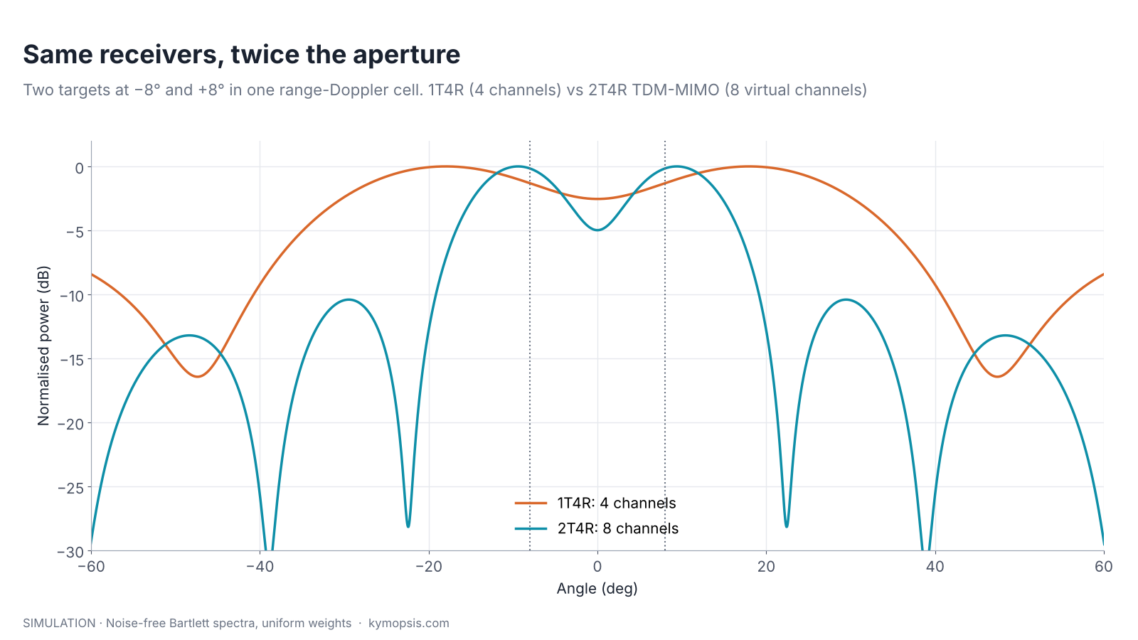
It does not create signal energy. With TDM, the energy collected per frame is the same as a single transmitter firing every chirp, it is just spread over more virtual channels; SNR after angle processing is therefore about the same as the single-transmitter radar, while resolution is better. Only schemes that keep several transmitters on at once, BPM and DDM, collect more energy. And unlike a phased array, a MIMO radar does not focus its transmit power in one direction; it illuminates the whole field of view all the time. Focusing power, and the transmit-side beamforming that does it, is the subject of the beamforming and phased array chapter.

Virtual channels are also only as good as the calibration of the physical ones. A phase error on one transmitter appears on all N_RX of its virtual channels, and a TX–RX coupling path near the board adds a fixed echo at very short range on every channel.

Try it yourself: examples/ch14_mimo_virtual_array.py in the open-source radar-basics-sim repository runs the core simulation of this chapter; change the assumptions and see what moves.

MIMO on the 2T2R modules we sell

Two lamps and two eyes make four lamp-and-eye pairs. Put the four in a line and they read left and right more finely; arrange them in a square and they trade some of that for a rough sense of up and down.

Our 60 GHz AiP and PCB-antenna radar modules each have two transmit and two receive channels. Run as TDM-MIMO, 2T2R gives up to four virtual channels, twice the two physical receivers: a 1×4 line if the transmitters are spaced for it, or a 2×2 grid that trades azimuth aperture for an elevation estimate. The supplier datasheets state the channel count and a ±60° field of view in both planes but not the antenna coordinates or the MIMO scheme the firmware uses, so we do not quote a virtual-array layout or resolution for these boards. As a rule of thumb, four virtual channels resolve two people only when they are tens of degrees apart, which is why separation in range and Doppler comes first in any people-counting chain.

GitHub · Kymopsis /radar-basics-simView repository → B2B engineering · KymopsisNeed more angular resolution than 2T2R gives?Tell us the field of view, resolution and size budget. We scope multi-channel radar modules and antenna layouts for B2B projects.Describe your requirement

FAQ

What is a virtual array in MIMO radar?

The set of positions x_TX + x_RX for every transmitter–receiver pair. In the far field each pair’s echo has the phase of a single receiver at that position, so the angle processing can treat the N_TX·N_RX pairs as one larger array.

Does MIMO increase radar range?

TDM-MIMO does not: it spreads the same transmitted energy over more channels. BPM and DDM, with all transmitters on, collect N_TX times more energy and gain about 10·log10(N_TX) dB of SNR, which extends range modestly (range scales with the fourth root of SNR).

Why does TDM-MIMO reduce the maximum velocity?

Each transmitter repeats only every N_TX chirps, so the Doppler phase is sampled N_TX times less often and folds at a velocity N_TX times lower.

Which is better, TDM, BPM or DDM?

TDM is simplest and is the common default. BPM gains SNR at the cost of decoding. DDM gains SNR and avoids the between-slot motion error but shares the Doppler band and needs a scheme to identify each transmitter’s copy. The choice depends on the chip, the speeds involved and the processing budget.

Sources and method

• J. Li, P. Stoica (eds.), MIMO Radar Signal Processing, Wiley, 2009.
• Texas Instruments, “MIMO Radar” application report SWRA554 (ti.com): TDM, BPM and virtual arrays.
• Texas Instruments AWR1843BOOST evaluation module documentation (ti.com): an example of the 3T4R layout with a raised transmitter. We describe the arrangement only and draw our own figures.
• M. A. Richards, Fundamentals of Radar Signal Processing, 2nd ed., McGraw-Hill, 2014.

All figures are drawn from formulas or simulated with the Kymopsis Radar Principles scripts (ch14_mimo_virtual_array.py): generic textbook layouts in units of λ, 60.5 GHz, 4 GHz sweep, 50 µs per chirp. None shows a Kymopsis module’s antenna layout or measured data.