Radar Principles 9: FMCW Phase Measurement, From Centimetre Bins to Microns

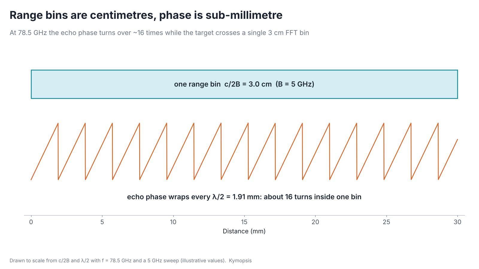
An FMCW radar with 5 GHz of sweep cannot separate two targets closer than 3 cm. The same radar can in principle, at high SNR and with a stable mount, resolve a single target moving by a few micrometres. Bandwidth sets how far apart two targets must be to be seen as two. Signal-to-noise ratio sets how precisely one target can be located, and the phase of the echo turns that SNR into sub-millimetre and even micrometre readings, because it goes through a full cycle every half wavelength: 1.91 mm at 78.5 GHz, 2.5 mm at 60 GHz.

The same principle is behind radar level gauges that quote millimetres, displacement monitoring on bridges and slopes, breathing and heartbeat research with 60 GHz modules, and angle finding with several receive channels. This article goes through how it works, how far it can be pushed, and what usually stops it.

Resolution, accuracy and precision are three different things

Think of darts. Two darts that touch can still be told apart if you look closely enough: that is resolution. Darts that land in a tight cluster are precise, even if the cluster sits off the bullseye; darts whose average lands on the bullseye are accurate, even if they scatter. A radar has all three, and each is set by something different.

Term	What it means	Set mainly by	Typical size at 76–81 GHz
Range resolution	Smallest gap at which two targets show up as two peaks	Sweep bandwidth B: ΔR = c/2B	3 cm with B = 5 GHz
Precision	Scatter of repeated readings of one target	SNR, and whether phase is used	From millimetres down to micrometres (see chart below)
Accuracy	Distance between the reading and the truth	Calibration, multipath, mounting, drift	Set by the installation; see the module datasheet

The numbers in the last column come from the formulas in this article with a full 5 GHz sweep. A real module may sweep less, and its datasheet figure is what counts for that module.

Where the phase comes from

Mark the valve on a bicycle wheel and roll the bike forward: the valve goes round once for every turn of the wheel. Where the valve points tells you exactly how far the wheel has rolled within one turn, but not how many turns it has made. The echo’s phase is that valve, and one turn is half a wavelength of target movement.

An FMCW radar transmits a chirp whose frequency rises linearly, then mixes the echo with the chirp still going out. A target at range R produces a beat tone. Its frequency is proportional to R, which is what the range FFT measures. Its phase is, to a good approximation,

φ = 4πR / λ  (plus a constant set by the hardware)

The factor 4π instead of 2π is there because the wave travels to the target and back. Move the target by λ/2 and the round trip changes by one whole wavelength, so φ goes once around the circle. At 78.5 GHz λ/2 is 1.91 mm; at 60 GHz it is 2.50 mm. Inside one 3 cm range bin the phase therefore wraps about 16 times. The FFT bin tells you roughly where the target is; the phase tells you where it is within a fraction of those 1.9 mm.

The phase itself, and why radars record it as I and Q, is the subject of chapter 2; the full derivation of the beat signal, including this phase term, is in chapter 5.

Step 1: find the peak between the bins

The range FFT gives samples at whole bins. A target almost never sits exactly on one, and its peak spreads over a few neighbouring bins in a known shape. Fitting that shape through the three largest samples, a parabola or a Gaussian on the log magnitude, puts the peak at a fraction of a bin. Zero-padding the FFT does the same job in a brute-force way. With a clean, strong echo, a level radar can get from a 3 cm bin to around a millimetre this way alone. Chapter 8 compares the interpolation methods and their limits in detail.

Step 2: read the phase at that peak

A clock’s hour hand tells you roughly what time it is; the minute hand tells you exactly, but only within the hour. You need both to read the time. The range peak is the hour hand, the phase is the minute hand.

Once the target’s bin is known, the phase of the FFT at that bin gives the fine position. But phase repeats every λ/2, so on its own it cannot say which 1.9 mm cycle the target is in. Two ways around that:

• Coarse plus fine. Use the interpolated peak to pick the cycle, then the phase to place the target inside it. This needs the coarse estimate to be good to better than about ±λ/4 (±0.95 mm at 78.5 GHz), which in turn needs enough SNR.
• Track over time. Measure many times per second and unwrap the phase from frame to frame. This works as long as the target moves less than λ/4 between two frames, and it gives relative motion rather than absolute distance. It is how displacement and vibration measurements are done.

The animation shows why phase is worth the trouble. A target moving by a hundredth of a range bin leaves the range profile unchanged, while the phase of its bin swings back and forth by more than 100°. Unwrapping that phase and multiplying by λ/4π recovers the motion. The same chain, applied to a chest wall instead of a vibrating plate, is the basis of the breathing measurements in chapter 11, and applied from one chirp to the next it becomes Doppler processing in chapter 10.

How fine it can get: the noise bound

A school ruler is marked in millimetres; a micrometer screw moves half a millimetre per turn and has a dial that reads hundredths of that. Bandwidth gives the radar a ruler; the carrier’s short wavelength gives it a micrometer.

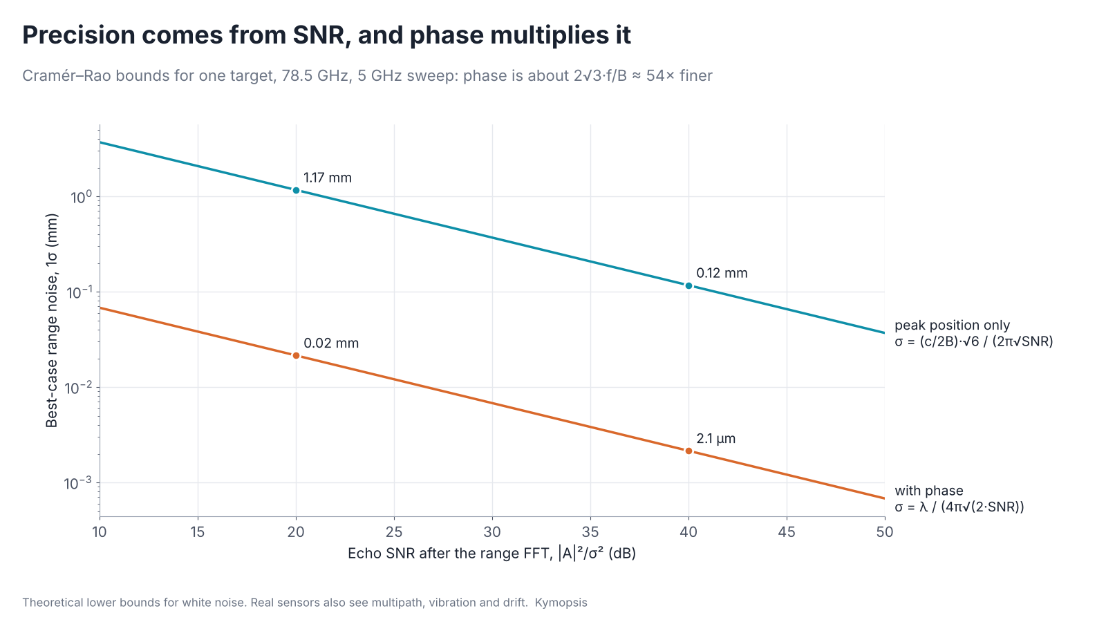
At 20 dB SNR the best case is about 1.17 mm from the peak position alone and 0.02 mm with the phase; at 40 dB, 0.12 mm and about 2 µm. Phase is roughly 2√3 · f_c/B ≈ 54 times finer for a 5 GHz sweep at 78.5 GHz. The carrier frequency is a much finer ruler than the bandwidth. One caution: the phase figure is for changes of distance. To read an absolute distance, the peak position must first pick the right phase cycle, which needs its error well inside ±λ/4 (±0.95 mm here), say three standard deviations. At 20 dB the 1.17 mm peak error is far too large for that; three standard deviations fit inside ±0.95 mm from about 31 dB, so absolute coarse-plus-fine ranging needs roughly 31–35 dB at the bound, more in a real installation.

The formulas behind the chart

For a single target in white noise, the Cramér–Rao bounds are:

• Peak position only: σ ≈ (c/2B) · √6 / (2π · √SNR)
• With phase: σ ≈ λ / (4π · √(2 · SNR))

SNR here is |A|²/σ² of the echo at its range bin after the FFT, the same definition for both lines. Their ratio is 2√3 · f_c/B. The phase bound assumes the bin is already known; if the coarse estimate picks the wrong λ/2 cycle, the error is a whole cycle, not a small scatter.

Both lines fall as SNR rises. That is why antenna gain matters for accuracy, not just for range. Sweep bandwidth is the other lever: the two 80 GHz level kits we sell measure ±2 mm (20 m kit) and ±4 mm at any distance (60 m kit, whose long-range waveform sweeps a narrower band). We go through that case, and why two boards with the same chip reach 20 m and 60 m, in Same 80 GHz chip, 20 m vs 60 m: why the antenna sets the range.

What stops you reaching the bound

A micrometer is no help if the table shakes, the part has warmed up, or something else leans against what you are measuring. Phase measurements fail in the same ways, usually long before noise sets the limit.

The chart is a floor, not a promise. In practice these usually dominate long before thermal noise does:

• Other echoes in the same bin. The phase you read is the phase of everything in that bin added together. A wall, a bracket or a second reflection a few centimetres away pulls the phase, and with it the reading. A narrow beam and a clean scene matter more than any algorithm.
• The mount moves. A sensor on a pole that sways by 0.1 mm reports 0.1 mm of target motion. For displacement work, the reference has to be stiffer than the motion you want to see.
• Temperature and drift. Oscillator, cable and PCB delays shift with temperature and add a slow phase drift. Long-term measurements usually watch a fixed reference target and subtract its drift.
• The air. Radio waves travel slightly slower in air than in vacuum, and the difference moves by a few to several tens of parts per million with temperature, pressure and humidity. One part per million over 100 m is 0.1 mm, which matters for long outdoor paths and not at all inside a small tank.
• Unwrapping errors. If the target jumps by more than λ/4 between frames, or the SNR dips, the unwrapped phase can slip by a full cycle and the result jumps by λ/2. The same quarter-wavelength limit sets the maximum unambiguous velocity (chapter 10); chapter 15 covers ways around it.

Where phase measurement is used

Level gauges

A liquid surface is close to an ideal phase target: one strong echo, slow movement, and nothing else at the same range if the beam is narrow. Industrial 80 GHz level radars quote millimetre accuracy from centimetre range bins using interpolation and, in many designs, phase. Foam, turbulence and condensation on the antenna lower the SNR and the precision with it.

Bridges, slopes and structures

Displacement monitoring turns the idea around: the radar looks at a fixed point on a structure, often a metal corner reflector bolted on for a strong echo, and tracks the phase over hours or months. Relative movement below a millimetre shows up as a slow change in phase. Interferometric radar systems for bridges, dams and landslide slopes are built on this, with careful compensation for the atmosphere and for the radar’s own drift.

Breathing and heartbeat research

Breathing moves the chest wall by millimetres, and the heartbeat adds a much smaller motion on top. Both are far below the range resolution of any small radar, but they are well within reach of the phase. Research setups pick the range bin of the person, unwrap its phase over time, and then filter it into a breathing band and a heartbeat band. The hard parts are the ones above: body movement swamps the tiny heartbeat signal, other people and objects share the bin, and SNR drops quickly with distance and angle.

This is research work. A radar module reading phase is not a medical device, is not for diagnosis or for safety monitoring, and our 60 GHz AiP radar sensor offers its breathing and heart-rate firmware on that basis only.

Angle finding with several receivers and MIMO

Put two receive antennas side by side and an echo from one side reaches one of them over a slightly longer path. The phase difference between the two channels gives the angle, and more channels, or the virtual channels of a MIMO radar, sharpen it. Chapter 12 works through it with numbers; all of it rests on the same phase measurement, which is why channel-to-channel phase calibration is one of the first jobs when bringing up a multi-channel radar.

Phase centres also explain a less obvious effect. When transmit and receive antennas sit apart and you put a lens in front of them, their beams point in slightly different directions. We show what that does to range in the level radar antenna comparison.

Try it on real hardware

The 80 GHz radar level sensor kit outputs distance over UART and can also return the echo curve (512 FFT bins), which is a good way to see a range peak, its neighbours and the effect of the antenna on a real target. The 60 GHz AiP sensor and the PCB-antenna development kit cover presence, gesture and breathing and heart-rate output for research.

Try it yourself: examples/ch09_phase_precision.py in the open-source radar-basics-sim repository runs the core simulation of this chapter; change the assumptions and see what moves.

GitHub · Kymopsis /radar-level-sensor-guiView repository → GitHub · Kymopsis /radar-basics-simView repository → B2B engineering · KymopsisBuilding a displacement or vital-sign prototype?Tell us the target, distance and resolution you need. We scope radar hardware, antennas and processing for B2B projects.Describe your measurement

Related: radar system design and radome design for 24–80 GHz radar, since a cover in front of the antenna adds its own near-range echo.

FAQ

If phase is so precise, why do level radars quote millimetres and not micrometres?

Because accuracy in a real vessel is limited by everything around the target: foam, waves, other echoes in the same bin, condensation, temperature drift and how the sensor is mounted. The phase bound is what the noise allows, not what the installation allows.

Can I get sub-millimetre resolution between two targets with phase?

No. Phase improves the precision of one target. Two targets closer than c/2B still fall in the same bin, and the phase you read is a mix of both. Separating them needs more bandwidth or angle information.

Do I need 80 GHz for phase measurement?

No. Any coherent FMCW radar has phase. A higher carrier makes λ/2 shorter, so the same phase noise means less displacement noise: 1.9 mm per cycle at 78.5 GHz against 2.5 mm at 60 GHz and about 6.2 mm at 24 GHz.

Can a radar module replace a medical monitor or a structural safety system?

No. Development kits like ours are for research, learning and prototyping. They are not medical devices and not certified safety equipment, and their output should not drive medical or safety decisions.

Sources and method

• D. C. Rife and R. R. Boorstyn, Single-tone parameter estimation from discrete-time observations, IEEE Trans. Information Theory, 1974 (Cramér–Rao bounds for frequency and phase).
• M. A. Richards, Fundamentals of Radar Signal Processing, 2nd ed., McGraw-Hill, 2014 (FMCW phase, interferometry).
• Texas Instruments, Introduction to mmWave Sensing: FMCW Radars (phase and displacement).
• Figures are simulations computed in Python from the formulas shown; code in Kymopsis/radar-basics-sim.