Radar Principles 19: 4D Imaging Radar and Point Clouds from Large MIMO Arrays

A conventional automotive radar sees a sign gantry 30 m ahead as a strong static echo in the lane, exactly what a stopped car looks like. A 4D imaging radar measures the gantry about 5.5 m above the road, so the car can drive under it. ‘4D’ means each detection carries four measured coordinates, range, radial velocity, azimuth and elevation, and the output is a point cloud rather than a short target list. It takes an array of tens to hundreds of virtual channels, which is why 4D radars are built from cascaded radar chips or large single chips, and why their processing chain is the whole of this series in one place.

This is chapter 19 of Radar Principles. It assembles the earlier chapters: the range-Doppler map, CFAR detection and tracking, MIMO virtual arrays and their ambiguities, and the super-resolution methods that imaging radars increasingly rely on. We keep to published principles and simulation; the numbers below describe our own simulated array, not any product.

What a 4D radar outputs

Picture a night photograph with no colours, made of a few hundred bright dots, where every dot also carries a tiny speedometer: the road and the gantry stand still, and the dots on a passing car show its speed. That is what a 4D radar hands over every frame: a cloud of points, each with a position, a height and a speed.

Each frame, a 4D radar reports a list of points, often hundreds to a few thousand in a real scene, each with x, y, z, radial velocity and signal strength. Downstream software clusters them into objects, tracks the objects over frames and classifies them, much as a lidar pipeline would. The radar’s advantages stay the same as in any FMCW radar: velocity measured directly in every point, operation in rain, fog, dust and darkness, and a sensor that hides behind a bumper. Its disadvantage against lidar is resolution: even a large radar array resolves around a degree, where a lidar resolves a tenth of that or better.

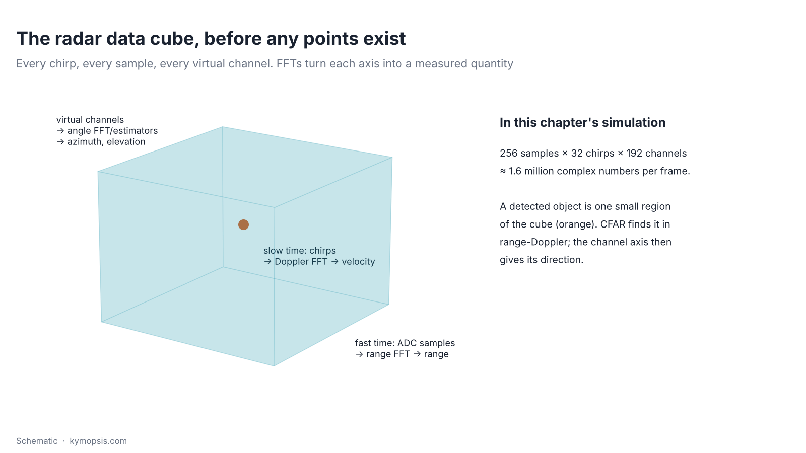
Before there are points there is a cube of numbers. Each chirp gives a row of ADC samples on each virtual channel; stacking the chirps of a frame and the channels gives three axes. The range FFT turns the sample axis into range, the Doppler FFT turns the chirp axis into velocity, and angle estimation turns the channel axis into direction. A point is one small region of that cube where something reflected.

Why it needs a big array

A bigger telescope mirror shows finer detail in the sky. To tell two cars side by side far down the road apart, a radar needs a much wider row of antennas than one chip carries, so several chips are joined into one long array.

Angle resolution is set by aperture: about 2/N radians for N elements λ/2 apart (angle chapter). To tell two cars in neighbouring lanes apart at 100 m, 3.5 m apart, needs about 2°, so N of 60 or more in azimuth. To separate a bridge from a car under it needs some elevation aperture as well. A single 3TX/4RX chip has 12 virtual channels, 8 of them in azimuth, which resolves about 14°.

The common answer is cascading: several radar chips on one board share a local oscillator and a frame trigger, so they act as one radar with all their transmitters and receivers. TI’s published 4-chip cascade reference design, for example, combines four 77 GHz transceivers into 12 transmitters and 16 receivers, uses 9 of the transmitters for an azimuth virtual array of 86 elements at λ/2 and offsets the other 3 vertically for elevation. We built a layout with the same published properties for this chapter’s simulation:

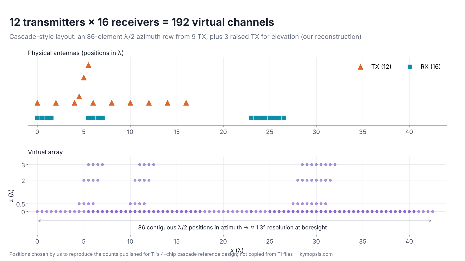
Three properties carry over to any such design. The azimuth row is long and dense, about 16.6 cm at 77 GHz, giving roughly 1.3° at boresight. Elevation comes from a few sparse rows, so it is coarser and prone to ambiguity; processing has to combine the rows carefully. And with 12 transmitters taking turns (TDM), each transmitter repeats only every 12 chirps: in our simulation the unambiguous velocity drops to ±3.2 m/s, far below road speeds, so velocity unfolding or another MIMO scheme (BPM or DDM) is not optional. Newer single-chip imaging radars integrate more channels per chip and increasingly use DDM or other simultaneous-transmit schemes for this reason.

From samples to points

Sorting a huge pile of post goes street first, then house, and only then do you read the names on the few letters left. A 4D radar sorts by range and speed first, keeps the few cells that hold something, and only then works out their direction.

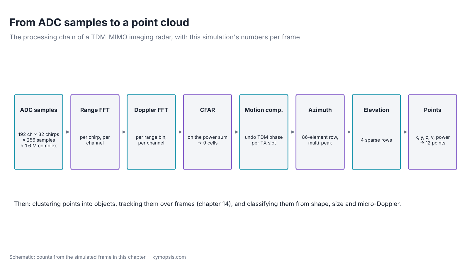
The chain is the series in order. Each of the 192 virtual channels gets a range FFT per chirp and a Doppler FFT per range bin, giving a range-Doppler cube. The power is summed over channels and CFAR picks the cells that hold something. Only those cells go through angle processing, which keeps the cost manageable: the angle steps run on a few hundred cells, not on millions.

For each detected cell, the TDM phase between transmit slots is removed using the measured velocity, as in the MIMO chapter. Then the angles: our simulation runs an azimuth spectrum over the 86-element row and keeps every peak within 12 dB of the strongest, because several reflectors (the bumper corners and lamps of the car) often share one range-Doppler cell and only angle can split them. For each azimuth peak, it removes the azimuth phase from all channels, averages each row and fits elevation across the four rows. That two-step approach is cheap and works because azimuth and elevation are measured by different parts of the array. Production radars refine it with 2D FFTs, super-resolution or sparse reconstruction to get more points per cell.

What the simulated frame contains, and what it gets

Radar 0.5 m above the road at 77 GHz, 1 GHz sweep (15 cm range bins), 20 µs ramps, 32 chirps per transmitter, 12TX/16RX TDM. Scene: the rear of a car at 18–18.6 m closing at 1.5 m/s (eight body reflectors on two lines and two wheels), a pedestrian 11 m ahead and 3.5 m to the left walking away at 1 m/s (two reflectors), a sign gantry 30 m ahead with three reflectors 5.5 m up, and five guard-rail posts on the right. Result: 9 CFAR cells and 12 points. The three gantry points come out at 4.7, 5.5 and 6.2 m (true 5.5 m, mean 5.5 m): with only 3 λ of elevation aperture and the three reflectors sharing range cells, each height is good to about a metre. The guard-rail posts land within a few centimetres in x and y, the pedestrian as one point, and the car as three points across its width: its reflectors are about 0.5 m apart, close to the 42 cm azimuth resolution at that range, so some merge, and the weaker wheel echoes fall below the 12 dB peak threshold. The script ch19_4d_point_cloud.py prints the full list.

From points to objects

Stars are only dots until you join them into constellations. Points from one car, one person or one bridge are grouped into objects and followed from frame to frame, and only then does the car know what is out there.

A point cloud is not yet a perception output. Points are clustered into objects (DBSCAN on position and velocity is the usual first step), each cluster gets a box and a velocity, and a tracker (chapter 16) carries objects across frames, which also suppresses the false points that CFAR lets through. Classification uses the cluster’s extent, its number of points, its radar cross-section and its micro-Doppler: a pedestrian’s swinging limbs spread their points over a range of velocities, a car’s do not. Machine-learning detectors that work directly on radar points or on the range-Doppler-angle cube are common in current research.

Two radar-specific problems remain hard. Multipath under and around vehicles creates ghost points, sometimes below the road surface or behind walls. And the sparse elevation rows produce elevation ambiguities and ground reflections that must be suppressed before a bridge is trusted to be a bridge.

Try it yourself: examples/ch19_4d_point_cloud.py in the open-source radar-basics-sim repository runs the core simulation of this chapter; change the assumptions and see what moves.

Where we stand

We work at the small end of this: boards with two transmitters and two receivers. Think of them as a pair of eyes for one room, not a telescope for a motorway.

We do not sell 4D imaging radars or cascade boards, and this chapter describes no product’s performance. The same principles run, at a much smaller scale, in the modules we do offer: the 2T2R 60 GHz AiP radar has at most four virtual channels for angle, and the 80 GHz level radar kit works in 76–81 GHz and measures one distance precisely. If your project needs imaging-radar capability, tell us the scene and requirements and we will discuss what can be sourced and supported.

GitHub · Kymopsis /radar-basics-simView repository → B2B engineering · KymopsisPlanning a project that needs a radar point cloud?Describe the scene, range, resolution and volume. We scope radar hardware and processing for B2B projects.Describe your project

FAQ

What does 4D mean in 4D imaging radar?

Each detection carries four measured values: range, radial velocity, azimuth and elevation. Conventional automotive radars measure the first three, or measure elevation only coarsely.

How many antennas does a 4D radar need?

Enough virtual channels for about a degree of azimuth resolution and some elevation aperture, typically around a hundred or more virtual channels, from cascaded chips or large single chips running MIMO.

Is a 4D radar as good as a lidar?

No on angular resolution, where lidar is roughly ten times finer. Yes or better on direct velocity measurement, weather robustness and concealed mounting. Many vehicle programmes use both.

Why does TDM-MIMO limit a 4D radar’s maximum velocity?

Each of the N transmitters fires only every N chirps, so the Doppler phase is sampled N times less often and folds at N times lower velocity. Imaging radars use velocity unfolding, staggered chirp timing or DDM to get around it.

Sources and method

• Texas Instruments, “Imaging Radar Using Cascaded mmWave Sensor Reference Design” (TIDEP-01012) design guide (ti.com): 4-chip cascade, 12 TX / 16 RX, 86-element azimuth virtual array. We cite its published properties and draw our own layout.
• Texas Instruments, “MIMO Radar” application report SWRA554 (ti.com).
• M. Ester et al., ‘A density-based algorithm for discovering clusters (DBSCAN)’, KDD, 1996.
• M. A. Richards, Fundamentals of Radar Signal Processing, 2nd ed., McGraw-Hill, 2014.

All figures are simulated with the Kymopsis Radar Principles scripts (ch19_4d_point_cloud.py, built on the shared FMCW simulator): point reflectors, a 77 GHz 12TX/16RX TDM array with our own antenna positions, 2-D CA-CFAR, Doppler compensation and two-step angle estimation. No figure shows a real product or real data.