



Every precision figure in the rest of this series, how finely a radar can place a target inside a range bin, how small a vibration it can see, how accurately it measures an angle, comes back to one number: the signal-to-noise ratio (SNR). This chapter builds that number from the radar equation, shows where the noise comes from, and explains why radars add up many chirps before deciding that something is there.
The radar equation
A radio wave spreads out like the light from a torch. At twice the distance the same energy covers four times the area, so a person there catches a quarter as much; the echo spreads out again on the way back, another quarter. Twice as far therefore means sixteen times weaker, and a fingernail-sized radar chip sees metres, not the hundred kilometres of an airport radar. To see twice as far you need sixteen times more from somewhere: transmit power, antenna gain on both trips, a longer listen by adding chirps, or simply a bigger target.
Follow the power. A transmitter sends Pt through an antenna with gain Gt. At range R the power density is PtGt/(4πR²), the 1/R² spreading from chapter 1. The target intercepts some of it and re-radiates as if it had an effective area σ, its radar cross-section. The returning wave spreads again, so at the radar it has density PtGtσ/((4π)²R⁴). The receive antenna collects it over an effective area Grλ²/(4π). Multiplying it out:
Pr = Pt · Gt · Gr · λ² · σ / ((4π)³ · R⁴ · L)
L collects everything else that is lost: cables and transitions, the radome, atmospheric absorption, and processing losses such as window functions. Each term is a lever a designer can pull, and the R⁴ is the one nobody can avoid: doubling the range costs 12 dB, ten times the range costs 40 dB.
Why λ² appears even though the target does not care about wavelength
It comes from the receive antenna. An antenna of gain G has an effective capture area Ae = Gλ²/(4π). For a fixed gain, a shorter wavelength means a smaller antenna and therefore less collected power. If instead you keep the antenna size fixed and go up in frequency, the gain rises as 1/λ² and more than compensates. That is the trade between small modules at 60 GHz and the large lens antennas on 80 GHz level gauges (chapter 4).
Radar cross-section
A mirror tilted towards you flashes sunlight into your eyes; tilt it a little and it goes dark, while a small bicycle reflector sends light straight back from almost any angle. How bright a target looks to a radar depends on its shape and angle in the same way, much more than on its size.
σ is not the physical size of the target. It is the area of an ideal reflector that would send back the same power. A flat metal plate facing the radar has an RCS far larger than its area; the same plate tilted by a few degrees reflects the energy away and almost disappears. Corner reflectors, three plates at right angles, send energy back towards the source from a wide range of angles and are used as calibration targets.
| Target (millimetre-wave, rough order of magnitude) | Typical σ |
|---|---|
| Person, front view | ≈ 0.1–1 m² |
| Hand | ≈ 0.01 m² |
| Car, front | ≈ 10–100 m² |
| Small corner reflector (5 cm edge, 60 GHz) | ≈ 1 m² towards the radar |
| Calm liquid surface in a tank, at normal incidence | large, but drops quickly with surface waves or foam |
These values are only orders of magnitude: RCS changes strongly with aspect angle, frequency and posture, and, as chapter 3 showed, fluctuates when many scatterers add. Treat any single number with care.

Where the noise comes from
Turn a radio between stations and you hear a hiss. Every receiver has a hiss of its own, even with nothing to receive, and an echo is only useful if it stands out from it.
Any resistor at temperature T produces random voltage, and so does every receiver. Its power over a bandwidth B is kTB, with Boltzmann’s constant k. At the reference temperature T₀ = 290 K this is −174 dBm per hertz of bandwidth. A real receiver adds its own noise on top, described by the noise figure F: the factor by which it makes the SNR worse. Millimetre-wave radar chips commonly have noise figures of around 10–15 dB, so the effective noise level is about −174 + 12 = −162 dBm/Hz.
What is this noise, physically? The electrons in any conductor jiggle with heat, and each jiggle is a tiny random current. Added up, they make a hiss with no particular frequency: equally strong at every frequency, which is why it is quoted per hertz and why a receiver that listens to a narrower band collects less of it. That is the first lesson for radar design: noise power grows with bandwidth, so anything that narrows the effective bandwidth, such as a longer chirp or the FFT itself, lowers the noise a target has to beat. Decibel arithmetic (chapter 1) makes this easy: in a 1 MHz bandwidth, kTB is −174 + 60 = −114 dBm.
The second lesson is about where in the receiver the noise figure is decided. A receiver is a chain: low-noise amplifier (LNA), mixer, IF amplifiers, ADC. Each stage adds noise, but noise added late in the chain is compared with a signal that the earlier stages have already amplified. The total noise factor (F as a ratio, not in dB) is given by Friis’ formula:
Ftotal = F1 + (F2 − 1)/G1 + (F3 − 1)/(G1G2) + …
With a first stage of 15 dB gain, a noisy mixer behind it barely matters: its contribution is divided by 31. That is why the first amplifier, and any loss in front of it, set the noise figure. A lossy radome or a long feed line before the LNA adds its loss in decibels directly to the noise figure, one reason radome design matters for range.
Friis’ formula with numbers
Take an LNA with 5 dB noise figure and 15 dB gain (F1 = 3.16, G1 = 31.6), followed by a mixer with 12 dB noise figure (F2 = 15.8). F = 3.16 + 14.8/31.6 = 3.63, or 5.6 dB: the mixer adds only 0.6 dB. Swap the order and F = 15.8 + 2.16/1 ≈ 18, or 12.6 dB, assuming the mixer has no gain. Put a 2 dB loss in front of the LNA and the total becomes 7.6 dB. Single-chip radars integrate the whole chain, so the datasheet gives one overall noise figure.
Thermal noise is not the only floor. Phase noise of the oscillator, leakage from transmitter to receiver, and reflections from the radome all raise the noise floor close to strong targets. For a single faint target in an empty scene, thermal noise dominates; in a cluttered room, the strongest objects often set the limit.
SNR for an FMCW radar
A faint voice is easier to pick out of a hiss if you listen longer: the voice keeps adding up while the hiss averages out. An FMCW radar listens for the whole chirp, so a longer chirp lifts the echo further above the noise.
An FMCW radar does not look at the raw receiver output. It takes an FFT over the samples of each chirp (chapter 6), and each FFT bin has an effective noise bandwidth of about 1/T, where T is the time over which the samples were taken. The echo energy, meanwhile, is collected over that whole time. The SNR in the target’s range bin after one chirp is therefore
SNR = PtGtGrλ²σ · T / ((4π)³ R⁴ · kT₀ · F · L)
Read it as energy over noise density: a longer sampling time collects more echo energy. That is the first reason radars integrate, and leads straight into the next section.
Integration: why radars add chirps
A long-exposure photo of the night sky shows stars the eye cannot see: their light piles up frame after frame, while the random grain does not. Adding chirps does the same for a faint echo.
Send N chirps at a target that does not move much and the echo in its range bin comes back with the same amplitude and nearly the same phase every time. Add the N complex values: the echo grows N times in amplitude, N² in power. The noise is random from chirp to chirp, so its power grows only N times. The SNR improves by a factor N, or 10·log10(N) dB.
In practice this addition happens inside the Doppler FFT (chapter 10): a target moving at constant speed lands in one Doppler bin with the full gain, even though its phase changes from chirp to chirp. Multiple receive antennas add another factor when they are combined coherently towards the target’s direction (chapter 14). Adding magnitudes instead of complex values, called non-coherent integration, also helps but gains less, roughly between √N and N depending on the SNR per look.
How much SNR is enough to detect
A lifeguard scanning the waves must decide when a bump is a swimmer’s head and not a wave. Set the bar too low and every wave is an alarm; set it too high and a real swimmer is missed. A radar’s detection threshold is that bar.
A radar decides that something is there when a cell rises above a threshold. Set the threshold too low and noise alone crosses it now and then, a false alarm; too high and real echoes are missed. As a rule of thumb, a steady target needs about 13 dB of SNR in one look to be detected 90% of the time while noise crosses the threshold only once in a million cells, and a target whose echo fluctuates, such as a person, needs about 21 dB. Chapter 16 shows where these numbers come from and how real radars set the threshold.
SNR sets precision
Point a laser pen at a wall with a shaky hand and the dot dances in a small cloud; steady the hand and the cloud shrinks. A strong echo against weak noise is the steady hand.
Detection is a yes/no question. Measurement is a how-much question, and here SNR matters even more. The uncertainty of a frequency estimate, and therefore of range, velocity and angle, shrinks as 1/√SNR. The picture behind it is the I/Q plane of chapter 2. The echo is an arrow; noise adds a small random arrow to its tip, so the tip wanders inside a little cloud. The stronger the echo compared with the cloud, the less the arrow’s angle and length wobble. In numbers, the phase of a phasor buried in noise wobbles by about 1/√(2·SNR) radians. At 20 dB SNR that is about 4°, or 28 µm at 60 GHz; at 40 dB it is 0.4°, or 3 µm.
Chapter 8 uses this to explain how a level radar resolves millimetres inside a range bin of several centimetres, and chapter 9 to explain micrometre phase ranging. In both cases the precision is bought with SNR.
A worked example
With illustrative parameters for a 60 GHz module, 10 dBm transmit power, 8 dBi antennas, 12 dB noise figure, 3 dB losses and 40 µs chirps, the radar equation gives:
| Target | Range | SNR, one chirp | SNR, 64 chirps |
|---|---|---|---|
| Person (σ = 1 m²) | 1 m | 62 dB | 80 dB |
| Person (σ = 1 m²) | 3 m | 43 dB | 61 dB |
| Person (σ = 1 m²) | 10 m | 22 dB | 40 dB |
| Hand (σ = 0.01 m²) | 3 m | 23 dB | 41 dB |
These are upper bounds from the textbook equation. Real modules lose margin to antenna patterns off broadside, clutter, multipath fades and implementation losses, which is why datasheet ranges are far shorter than the point where the curve crosses 13 dB. Use the formula to compare designs and to understand how precision scales, not to promise a range. Our product pages quote ranges from the module datasheets only.
The calculation is a few lines in the open-source radar-basics-sim library; change power, gain or RCS and rerun it.
Try it yourself: examples/ch07_radar_equation.py in the open-source radar-basics-sim repository runs the core simulation of this chapter; change the assumptions and see what moves.
-

80 GHz Radar Level Sensor Development Kit, 76–81 GHz, 20 or 60 Meter Range
From $99.00Reset options60-meter kit, horn + lens20-meter kit, lens radomeSelect options This product has multiple variants. The options may be chosen on the product page -
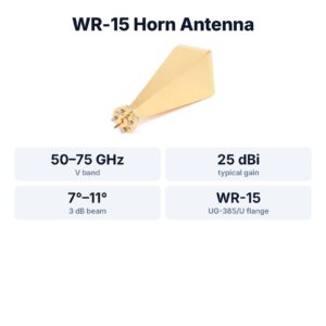
WR-15 Standard Gain Horn Antenna, 50–75 GHz, 25 dBi
$1,299.00 Buy Now
FAQ
Why does radar range only grow with the fourth root of power?
Because received power falls as 1/R⁴. Sixteen times the transmit power, 12 dB, only doubles the range for the same SNR.
Is a higher frequency radar always shorter range?
Not by itself. For the same antenna gain, the λ² term favours lower frequencies; for the same antenna size, higher frequencies win because the gain rises. Absorption matters only at long range or in rain.
What is a good SNR for a radar measurement?
For detection, 13–20 dB depending on how much the target fluctuates. For precise ranging or phase measurement, the more the better; precision improves by a factor of about 3 for every 10 dB.
Does averaging more frames always help?
Only while the target and the scene stay the same. A moving target spreads over Doppler bins, and slow drift adds errors that averaging cannot remove.
Sources and method
- M. I. Skolnik, Introduction to Radar Systems, 3rd ed., McGraw-Hill, 2001 (radar equation, RCS, detection).
- M. A. Richards, Fundamentals of Radar Signal Processing, 2nd ed., McGraw-Hill, 2014 (integration gain, Swerling models).
- D. K. Barton, Radar Equations for Modern Radar, Artech House, 2013.
- W. Albersheim, “A closed-form approximation to Robertson’s detection characteristics”, Proc. IEEE, 1981.
- Figures and animations are computed in Python from the formulas shown; the simulation code is open source in Kymopsis/radar-basics-sim. RCS values are rough orders of magnitude from the radar literature, not measurements. Figures marked SIMULATION are not measurements of a product.