Radar Principles 12: Angle of Arrival from a Phase Difference

Put two receive antennas half a wavelength apart, 2.48 mm at 60.5 GHz, and an echo from 30° off boresight reaches one of them 1.24 mm later than the other. The radar cannot time that directly, but it can read it as a phase difference of exactly 90° between the two channels. That phase difference, Δφ = 2π·d·sin θ/λ, is how most FMCW radars with more than one receiver measure angle, from a two-channel 60 GHz presence sensor to an automotive imaging radar with hundreds of virtual channels.

This is chapter 12 of Radar Principles. The range chapters ended with the phase of one range bin (phase measurement, from centimetre bins to microns); the velocity chapters used the phase change from chirp to chirp. Angle uses the third place a phase can change: from one antenna to the next.

A path difference you read as a phase difference

When someone calls you from the left, the sound reaches your left ear first and your right ear a fraction of a millisecond later, and your brain turns that gap into a direction. A radar does the same with two receiving antennas a few millimetres apart: an echo from a person off to one side reaches one antenna slightly before the other. With antennas 2.5 mm apart at 60 GHz, a person 30° to the side makes one path longer by a quarter of a wave.

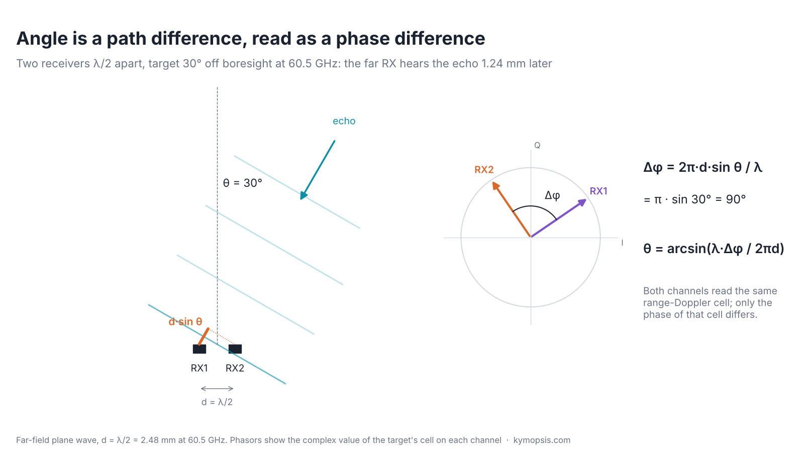
At a few metres, a target is far enough away that its echo arrives at the antenna board as a plane wave: flat wavefronts, all travelling in the same direction. If that direction is tilted by θ from the board’s normal (boresight), the wavefront touches one receive antenna first and the other a little later. The extra path is the antenna spacing projected onto the arrival direction, d·sin θ.

A path of one wavelength is one full turn of phase, so the extra path becomes a phase offset between the two channels:

Δφ = 2π · d · sin θ / λ   ⇒   θ = arcsin( λ · Δφ / (2π · d) )

Note that this is the one-way path. In range, the echo phase changes by 4πR/λ because the wave goes out and back. In angle, the transmit path is the same for both receivers and only the last leg differs, so the factor is 2π, not 4π.

A worked example makes the formula concrete. At 60.5 GHz the wavelength is 4.96 mm, so two receive antennas half a wavelength apart sit 2.48 mm apart. A target 30° to the side makes the far antenna’s path longer by 2.48 mm × sin 30° = 1.24 mm, a quarter of a wavelength, which is a quarter turn of phase: 90°. The radar works backwards. It measures 90° between the two channels, divides by 360° to get a quarter wavelength of extra path, divides by the spacing and takes the arcsine: 30°.

Your ears do the same with sound: a voice to your left reaches the left ear a fraction of a millisecond earlier. Radio waves are so fast and so short that the radar compares phase instead of arrival time, using the I/Q measurement from chapter 2. Because the antennas are only millimetres apart, the whole time difference is a few picoseconds; phase is the only practical way to see it.

The phase difference does not depend on range, velocity or the strength of the echo. It depends only on the geometry, which is why it works so well: a target walking towards the radar changes the phase of both channels by the same amount, and the gap between them stays put.

Where the two phases come from

Picture two microphones recording a choir. To tell which way the tenor stands, you first pick out the tenor’s voice on each recording, and only then compare when it arrives at each microphone. A radar works the same way: it first sorts every echo into its own range-and-speed box on each channel, and then compares the two channels inside that box.

A radar does not compare raw ADC samples between antennas. It runs the range FFT and the Doppler FFT on each receive channel separately, which gives one range-Doppler map per channel. A target appears in the same cell of every map, because range and velocity are the same for all the antennas. The magnitude of that cell is the same on each channel; its phase is not.

So angle estimation is a step after detection: find the peak cells, take the complex value of each cell on every channel (the snapshot), and estimate the angle from that short vector. With two channels the estimate is the phase of x₂·x₁^*. With more channels it becomes a third FFT, the angle FFT, across the channels. Doing it after the range and Doppler FFTs is not just bookkeeping: those FFTs have already integrated hundreds of samples and dozens of chirps, so the snapshot has far better SNR than any single ADC sample.

Because angle is needed only at detected cells, a radar short of processing power does not have to run the full range-Doppler FFT on every channel. One channel runs it and feeds the CFAR detector (chapter 16); the other channels compute their value only at the detected cells with a single-bin DFT, which gives the same complex number for a fraction of the work, and the phase difference between channels then gives the angle. Chapter 21 works through it.

Spacing and the field of view

Two ears close together never mix up left and right. Put them far apart and a sound could arrive a whole wave late at one ear, which looks exactly like arriving on time: two directions would fit the same reading. Keeping the antennas within half a wave of each other rules that out.

Phase is only known modulo 360°. A reading of +90° could also be −270° or +450°, and if those values are reachable for some angle in front of the radar, the angle is ambiguous. With spacing d the phase gap spans ±2π·d/λ over ±90°, so the gap stays within ±180°, and the angle stays unique, only while d ≤ λ/2.

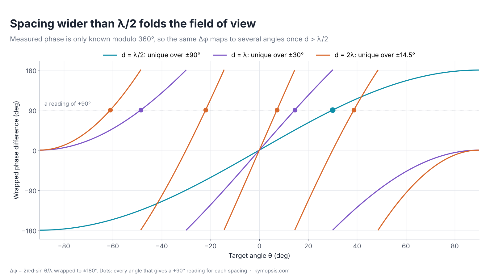
That is why λ/2 is the default element spacing in radar arrays. Wider spacing is not useless: the curve gets steeper, so the same phase noise gives a smaller angle error, and a longer baseline helps resolution. Designs that use it either restrict the field of view with the antenna pattern (a beam of ±14° behind a 2λ pair rarely sees the folded angles) or combine a wide baseline for precision with a λ/2 pair to pick the right fold. The same folding shows up as grating lobes in larger arrays, which come back in the MIMO and beamforming chapters.

In practice the patches themselves are about λ/2 across, so λ/2 spacing is close to the tightest layout possible. At 60 GHz that is 2.48 mm, at 77 GHz 1.95 mm, at 24 GHz 6.2 mm. Spacing in an antenna-in-package (AiP) chip is set by the package, which is one reason AiP radars are so small.

Precision of one angle reading

Telling where a sound comes from is easiest when it is in front of you: turn your head a little and the gap between your ears changes a lot. A sound from far to the side barely changes the gap as you turn, so your guess gets vague, and a faint sound makes it vaguer still. Radar angle behaves the same: sharpest straight ahead, blurrier towards the edges, and noisier when the echo is weak.

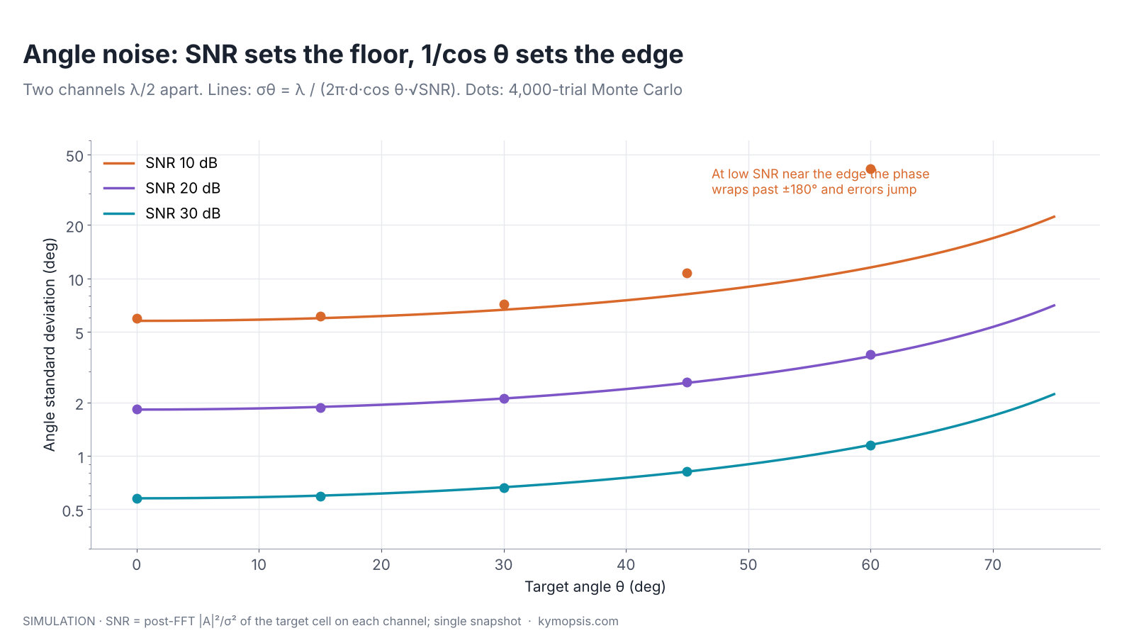
The phase of each channel carries noise. With a post-FFT SNR (|A|²/σ²) on each channel, each phase has a standard deviation of about 1/√(2·SNR) radians, and the difference of two independent phases about 1/√SNR. Dividing by the slope of the Δφ(θ) curve turns that into an angle:

σ_θ ≈ λ / (2π · d · cos θ · √SNR)

Post-FFT SNR per channel	θ = 0°	θ = 30°	θ = 60°
10 dB	5.8°	6.7°	11.5° (simulation: much worse, phase wraps)
20 dB	1.8°	2.1°	3.7°
30 dB	0.58°	0.67°	1.2°

Two things stand out. First, every 20 dB of SNR buys a factor of ten in angle precision, the same square-root law as in range. Averaging over more chirps or several frames raises the SNR and so tightens the angle, as long as the target holds still. Second, precision falls off as 1/cos θ: at 60° a target moving by one degree changes the phase gap only half as much as at boresight. A module datasheet that states a ±60° field of view, as the ones we sell do, does not say the angle is equally good across it; the edges are worse by about a factor of two even before the antenna gain drops there.

Where the 1/√SNR comes from, and when it stops holding

Write each channel as x_k = A·e^jφ_k + n_k with complex white noise of variance σ². For high SNR the phase error of one channel is the noise component perpendicular to the phasor divided by |A|, which has variance σ²/(2|A|²) = 1/(2·SNR). The two channels’ noise is independent, so the phase difference has variance 1/SNR. The slope dΔφ/dθ = 2π·d·cos θ/λ converts it to angle. This is the Cramér–Rao bound for two elements; for N elements λ/2 apart it falls roughly as N^−3/2, because more elements add both SNR and aperture.

The linearisation fails when the phase noise is no longer small compared with the margin to ±180°. Near θ = 60° the true phase gap is already 156°; at 10 dB SNR a noise excursion of 25° pushes it past 180°, the reading wraps to the other side and the estimate jumps by tens of degrees. That is the threshold effect in the simulated dots.

Two targets in one cell

When two people talk at once from slightly different places, you hear one blended voice from somewhere in between, or even off to one side of both. Two antennas hearing two echoes in the same box get the same muddle: they can only report the direction of the mixture.

Everything above assumes one target per range-Doppler cell. Two people standing at the same distance and both still, or a person and a chair behind them, put two echoes into one cell. The snapshot is then the sum of two phasor pairs, and two channels can only report one angle: whatever the phase of the sum says.

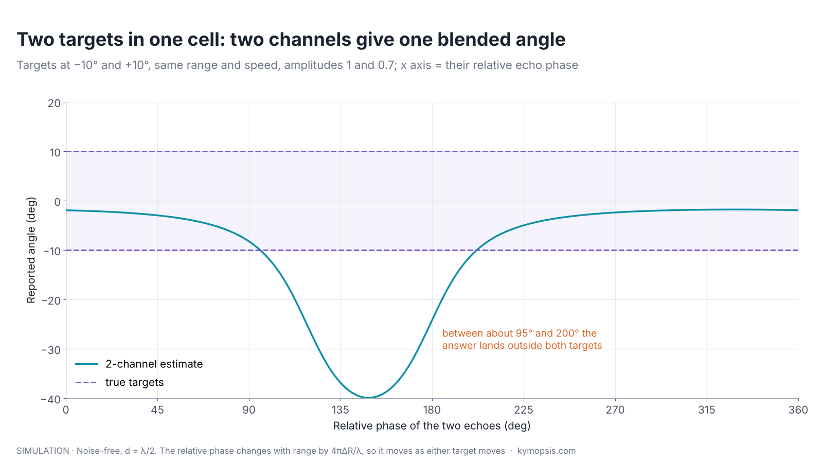
The result is not even a sensible average. It depends on the relative phase of the two echoes, which changes by a full turn for every λ/2 of range difference, 2.5 mm at 60 GHz. So a person breathing next to a static reflector produces an angle that wobbles by tens of degrees. Two remedies exist. Separate the targets in another dimension first: a moving person and a static chair land in different Doppler cells, which is why static-clutter removal comes before angle estimation in presence sensors. Or add channels, so that the snapshot has enough elements to resolve two directions.

More channels: from one angle to an angle spectrum

Two ears tell you roughly where one sound comes from. A long row of microphones can pick out several voices at once and point at each, and the longer the row, the closer two voices can stand and still be told apart.

With N channels on a λ/2 grid, the snapshot is N complex values, and an FFT across them gives an angle spectrum: power versus sin θ, with one peak per direction. This is the same Fourier relationship as the range and Doppler FFTs, applied across space instead of time.

The width of each peak, and so the angle resolution, is set by the aperture: about λ/(N·d) radians at boresight, or 2/N for λ/2 spacing. That is 57° for two channels, 29° for four, 14° for eight. Like range resolution, it is a property of the array, not of the SNR: averaging more frames sharpens the position of a single peak but does not split two peaks that the aperture cannot separate. Within its own peak, though, a single target’s angle can still be refined to a small fraction of the resolution by interpolation, exactly as with the range bin.

Getting N large is the subject of later chapters. MIMO radar multiplies transmitters and receivers into a larger virtual array. Beamforming weighs the channels to steer and shape the beam. Super-resolution methods such as MUSIC split peaks closer than 2/N, at a price in SNR and robustness.

What goes wrong on real boards

Wear a hat pulled over one ear and every sound seems to come from a slightly wrong direction until you get used to it. Radar receivers have the same quirks: each receive path adds its own small delay, an uneven cover adds another, and an echo off a wall seems to come from the wall.

The formula assumes identical channels. On a real board each receive path adds its own fixed phase: different trace lengths, mixer and filter tolerances, and the package. A 10° mismatch between two channels shifts every reading by about 3.2° at boresight and 6–7° at 60°. Radar SoCs therefore store per-channel phase and gain corrections, measured once against a corner reflector at a known angle, usually boresight, in a quiet room or chamber.

Other errors worth knowing about:

• The cover in front. A radome or housing that is not uniform across the antennas adds a different phase to each channel and bends the apparent angle. The radome chapter covers wall thickness and tilt; for angle work, keep the cover parallel to the board and the same thickness over all elements.
• Mutual coupling. Antennas λ/2 apart pick up part of each other’s signal, which distorts the phase gap, mostly at wide angles. Calibration at several angles, not only boresight, reduces it.
• Multipath. An echo that bounces off a wall arrives from a different direction and lands in a nearby range cell. It looks like a second target at the wrong angle, a ‘ghost’.
• Near field. The plane-wave model needs the target at more than about 2D²/λ, where D is the array size. For a small 60 GHz board that is a few centimetres; for a 10 cm imaging array at 77 GHz it is several metres.

Try it yourself: examples/ch12_angle_fft.py in the open-source radar-basics-sim repository runs the core simulation of this chapter; change the assumptions and see what moves.

Angle on the 60 GHz modules we sell

Our 60 GHz AiP radar module and PCB-antenna radar module both have two transmit and two receive channels (2T2R), and their supplier datasheets state a field of view of ±60° in both planes. The modules run their own processing, so you work with their outputs (a gesture code, or target information, depending on the firmware), not with raw phases. What this chapter tells you is how to read those outputs:

• Expect angle noise to grow towards the edge of the ±60° field and to shrink when the target is closer and stronger. Mount the board so the area you care about is near boresight.
• Two people at the same distance from the board and moving the same way are hard to separate with two receivers; their positions blend. Different distances or different motion help.
• A cover in front of the module shifts angles if it is not flat and uniform over the antenna area.

The Radar Desk Buddy project uses the AiP module’s target output to turn a servo towards the nearest person, which makes angle noise visible: you can watch the head jitter more when you sit far to the side. The datasheets do not give the antenna spacing, so we do not quote a resolution for these boards.

GitHub · Kymopsis /radar-desk-buddyESP32-S3 desk companion with a 60 GHz mmWave radar: eyes and figure follow you, local time and weather, Telegram messages. No soldering.CMIT licenseView repository → GitHub · Kymopsis /radar-basics-simView repository → B2B engineering · KymopsisNeed angle accuracy for your product?Tell us the field of view, distance and number of targets. We scope antenna layout, calibration and processing for B2B radar projects.Describe your application

FAQ

Why is the antenna spacing half a wavelength?

Because the phase gap 2π·d·sin θ/λ must stay within ±180° for every angle in front of the radar, or two angles give the same reading. With d = λ/2 the gap reaches ±180° only at ±90°. Wider spacing narrows the unambiguous field of view to ±arcsin(λ/2d).

Can a radar with one receive antenna measure angle?

Not from a single measurement. A scanning radar can, by turning a narrow beam and looking for the strongest echo, and a moving radar can, by synthetic aperture processing. A fixed single-channel FMCW module measures range and velocity only.

Why is the angle worse at the edge of the field of view?

The phase gap changes with sin θ, which flattens towards ±90°: at 60° a one-degree move changes the gap half as much as at boresight, so the same phase noise means twice the angle error. Antenna gain also drops at the edge, which lowers SNR.

Does more SNR improve angle resolution?

It improves precision, how tightly one target’s angle is measured, but not resolution, the smallest angle between two targets that still shows as two peaks. Resolution is set by the aperture, about 2/N radians for N channels λ/2 apart, unless super-resolution methods are used.

Why does my radar report a person at the wrong angle when they stand next to a wall?

Either the wall echo shares the person’s range-Doppler cell and blends with it, or a wall bounce arrives as a separate ghost from another direction. Both are multipath. Static-clutter removal and mounting away from large flat surfaces help.

Sources and method

• M. A. Richards, Fundamentals of Radar Signal Processing, 2nd ed., McGraw-Hill, 2014: array processing and angle estimation chapters.
• H. L. Van Trees, Optimum Array Processing, Wiley, 2002: Cramér–Rao bounds for direction of arrival.
• Texas Instruments, “Introduction to mmWave Sensing: FMCW Radars” training series, angle estimation module (ti.com).
• Supplier datasheets of the Kymopsis 60 GHz AiP and PCB-antenna radar modules, as published on the product pages.

All figures are computed or simulated with the Kymopsis Radar Principles simulation scripts (textbook FMCW model, 60.5 GHz, 4 GHz sweep, λ/2 spacing); none is measured data from the modules we sell. The script for this chapter, ch11_angle_phase.py, prints every number in the text and checks the simulated estimates against the formulas.