


Almost everything a radar measures is read from a phase or a frequency, and both live on a circle. Go once around and you are back where you started. A target just beyond the maximum range shows up near the radar, a car faster than the maximum velocity appears to drive backwards, and an antenna array with too wide a spacing sees the same target in several directions. These are ambiguities. This chapter collects the three of them, adds the one that MIMO radars create by tying velocity and angle together, and shows the standard ways to unfold each.
Why measurements wrap around
A clock face shows only twelve hours: three in the afternoon looks exactly like three at night. Anything a radar reads from a phase or a frequency sits on a dial like that, and to know which turn of the dial is the right one it needs a second clue, the way daylight outside the window tells you it is afternoon.
A sampled signal cannot tell a frequency f from f + fs, and a phase reading cannot tell φ from φ + 360°. Each of the radar’s three measurements is built on one of these:
- Range is a beat frequency sampled at the ADC rate (chapter 5).
- Velocity is a phase step between chirps, sampled once per chirp (chapter 10).
- Angle is a phase step between antennas, sampled once per antenna position (chapter 12).
In each case the span that can be measured without confusion is set by how densely the radar samples: in time for range, in chirps for velocity, in space for angle. Unfolding means bringing in a second, independent piece of information that tells which turn of the circle the target is really on.
Range ambiguity
Clap at a steady rhythm in a canyon: an echo from a far cliff that arrives after your next clap sounds like an echo from a near one. A radar can mistake a very distant echo for a close one in the same way. Change the rhythm and the impostor gives itself away: a true echo stays where it is, a false one jumps.
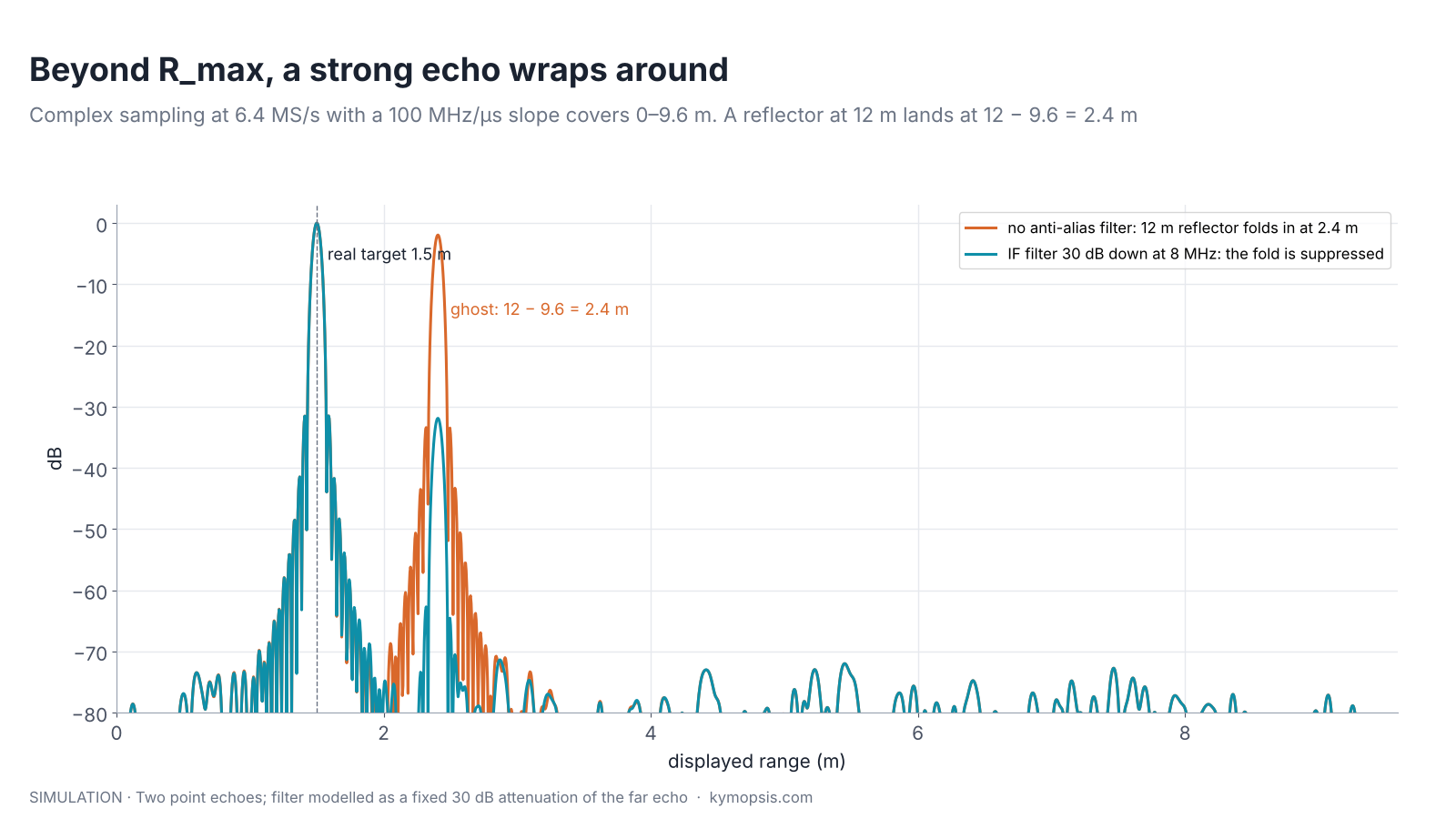
How far the range axis reaches depends on the sampling scheme (chapter 5). With real sampling at fs an FMCW radar covers beat frequencies up to fs/2, ranges up to Rmax = fs·c/(4S), and an echo from further away is mirrored back into the span. With complex (I/Q) sampling the span can reach fs, Rmax = fs·c/(2S), and an echo beyond it wraps to R − Rmax instead; how cleanly that extra half is usable depends on the I/Q balance (Radar Math 1). Either way the far echo shows up at a wrong range inside the span.
Short-range radars handle this mostly in hardware and configuration:
- Anti-alias filtering. The IF low-pass filter in front of the ADC attenuates beat frequencies above the span, so a far wall becomes much weaker than the targets of interest.
- Choosing the span. Set the slope and sample rate so that Rmax covers the whole room or tank, not just the region of interest. The radar equation helps too: far echoes are weak.
- Changing the slope. A real target stays at the same displayed range when the chirp slope changes. A folded one moves, because its displayed range R − Rmax depends on the slope. Alternating two slopes exposes it.
Pulse radars have a different range ambiguity, from echoes of an earlier pulse arriving after the next one is sent. FMCW radars at room scale do not suffer from it, because echo delays are tiny compared with the chirp.
Velocity ambiguity
Film a turning car wheel and at some speeds it seems to stand still or even spin backwards, because the camera catches each spoke just as the next one takes its place. A radar takes one snapshot of the echo’s phase per chirp, and a fast target can look slow, or as if it were moving away, in exactly the same way.
The Doppler FFT reads the phase step between chirps, 4πvT/λ. Once the step exceeds ±180°, the target appears at v − 2vmax (chapter 10 shows it on a range-Doppler map). At 60.5 GHz with a chirp every 50 µs, vmax is about ±24.8 m/s, plenty for people and hands. With a chirp every 250 µs it is ±4.96 m/s, and a running person or a swinging foot can exceed it. Four remedies are used, often combined:
- Shorter chirp interval. The direct fix, limited by the chirp duration and the processing load.
- Two chirp intervals. Measure with two different intervals and find the one velocity consistent with both, explained in the next section.
- Tracking. Range from frame to frame gives a coarse velocity (Δrange/Δt) that is unambiguous, though imprecise. It only has to be good enough to pick the right fold of the precise Doppler value, exactly like the coarse-plus-fine idea in chapter 9.
- Range migration. A fast target drifts across range bins within a frame; the direction and amount of drift tell which fold is right. It is used in long-frame, high-resolution radars.

Unfolding velocity with two chirp intervals
Two clocks that tick at different rates each repeat on their own, but the pair of readings together repeats only after a long time. A radar measuring with two chirp intervals gets two partial answers in the same way, and only one true speed fits both.
Suppose frame A uses a chirp interval T₁ and frame B uses T₂. Each frame knows the velocity only up to a multiple of its own span, 2vmax. List all candidates for each frame and look for the value that appears in both lists: that is the true velocity. Because the two spans differ, the candidates line up only at long intervals.

In the example a target at 30 m/s is measured as −19.6 m/s in frame A and −11.3 m/s in frame B. Only 30 m/s is in both candidate lists. This is the Chinese remainder theorem from number theory, and in radar it is often called staggered PRF or multiple PRF. The combined unambiguous span is much wider than either frame’s, limited in practice by noise: the candidates must agree within the velocity error, so the two spans should not be too close to each other.
Choosing the two intervals
If the spans are in a ratio p:q of small coprime integers, the combined span is q times the first span (or p times the second). Larger p and q extend it further, but candidates from the two lists then come closer to each other, so a noisy measurement may match the wrong pair. Practical designs pick ratios like 5:6 or 7:8 and check the match against a tolerance a few times larger than the velocity error from chapter 10.
Angle ambiguity and grating lobes
Walk past a row of streetlights behind railings and, from several spots, the lights line up between the bars in the same way. Antennas spaced more than half a wave apart see the same phase difference from several directions, and those extra directions are called grating lobes.
Two receive antennas d apart see a phase difference Δφ = 2π·d·sin θ/λ (chapter 12). If d is larger than λ/2, Δφ passes ±180° before θ reaches ±90°, and several directions produce the same reading. In an array, those extra solutions show up as grating lobes: copies of the main beam, just as strong, pointing elsewhere. Chapter 3 showed their origin in two-source interference.
The unambiguous field of view is |sin θ| < λ/(2d): ±90° for d = λ/2, ±30° for d = λ, ±14.5° for d = 2λ. Remedies:
- Keep λ/2 spacing where the full field of view matters. At 60 GHz that is 2.48 mm, which is why antennas-in-package are so compact.
- Let the antenna pattern hide the grating lobes. If each element only sees ±30°, a spacing up to λ can be used: the grating lobes fall where there is nothing to see.
- Two baselines. A short pair spaced λ/2 gives a coarse, unambiguous angle; a long baseline gives a precise but ambiguous one. The coarse value picks the fold, the same coarse-plus-fine idea as before.
- Non-uniform and sparse arrays. Irregular spacing spreads the grating lobes into lower side lobes, which MIMO virtual arrays exploit (chapter 14).
TDM-MIMO: when velocity spoils angle
Two people take turns photographing a passing car; if the car moves between their shots, comparing the photos makes it look shifted sideways. The radar undoes that shift using the car’s speed, and if the speed it uses has wrapped, the correction goes wrong.
A MIMO radar builds a large virtual array from a few transmitters and receivers (chapter 14). The simplest scheme, time-division multiplexing (TDM), lets the transmitters take turns: chirp 1 from TX1, chirp 2 from TX2, and so on. Two things follow.
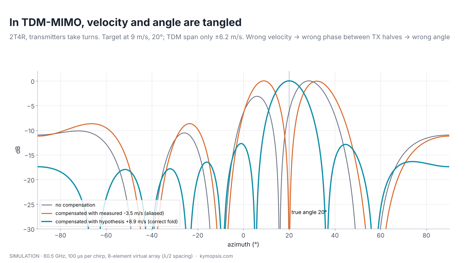
- The interval between chirps from the same transmitter grows to Ntx·Tc, so vmax shrinks by Ntx. With two transmitters and 100 µs chirps at 60.5 GHz it is only ±6.2 m/s.
- A moving target changes its phase between the TX1 chirp and the TX2 chirp. The virtual elements belonging to TX2 therefore carry an extra phase 4πvTc/λ that has nothing to do with angle. Left alone, it shifts and splits the angle spectrum.
The cure is to estimate the velocity first and remove the extra phase from each transmitter’s virtual elements before the angle FFT. That works only if the velocity estimate is unfolded correctly. The figure at the top shows a target at 9 m/s, beyond the ±6.2 m/s TDM span. It folds to 9 − 12.4 = −3.4 m/s; the Doppler peak actually lands near −3.1 m/s, because the target moves 11.5 cm during the frame and smears its peak by a bin or two. Compensating with that folded value splits the beam. Testing the Ntx possible folds and keeping the one that gives the sharpest single peak recovers the true angle and the velocity, as long as the true velocity lies within ±λ/(4Tc), the span of the un-multiplexed chirp rate (±12.4 m/s here); beyond that, the fold test is itself ambiguous and needs the methods above. Designs that place one virtual element of each transmitter at the same position can measure the extra phase directly from that overlap.
The compensation in code
import numpy as np
# snap: virtual-array values at the target's range-Doppler cell, ordered TX-major
# v_hat: Doppler velocity, Tc: time between consecutive chirps, lam: wavelength
def compensate(snap, v_hat, n_tx, n_rx, Tc, lam):
    k = np.repeat(np.arange(n_tx), n_rx)            # transmitter index of each element
    return snap * np.exp(-1j * 4 * np.pi * v_hat * k * Tc / lam)
# try the n_tx folds v_hat + m * 2 * v_max_tdm and keep the sharpest angle spectrum
Other MIMO schemes avoid part of the problem: Doppler-division (DDM) and binary phase modulation (BPM) transmit from all antennas at once with different codes, at the cost of other trade-offs covered in chapter 14.
Summary
| Dimension | What wraps | Unambiguous span | Common fixes |
|---|---|---|---|
| Range | Beat frequency vs ADC rate | fs·c/(2S) (complex) | IF filter, wider span, slope change |
| Velocity | Chirp-to-chirp phase | ±λ/(4T) | Shorter T, two intervals (CRT), tracking |
| Angle | Antenna-to-antenna phase | |sin θ| < λ/(2d) | λ/2 spacing, element pattern, two baselines |
| TDM-MIMO | Velocity phase between transmitters | ±λ/(4NtxTc) | Compensation with fold hypotheses, overlapped elements |
All four figures can be regenerated, with your own settings, from the ambiguity example in the open-source radar-basics-sim library. When you evaluate a module, read its antenna spacing and chirp timing from the datasheet and work out these spans before trusting a reading near their edges.
Try it yourself: examples/ch15_ambiguity.py in the open-source radar-basics-sim repository runs the core simulation of this chapter; change the assumptions and see what moves.
-

80 GHz Radar Level Sensor Development Kit, 76–81 GHz, 20 or 60 Meter Range
From $99.00Reset options60-meter kit, horn + lens20-meter kit, lens radomeSelect options This product has multiple variants. The options may be chosen on the product page -

60 GHz AiP Gesture & Presence Radar Sensor Module, Pre-flashed (57–64 GHz, 2T2R)
From $19.00Sensor onlySensor + USB-TTL adapter (3.3 V LDO)Reset optionsGesture recognitionPresence, ceiling mountPresence, wall mountPresence and fall events, ceiling mountBreathing and heart rate (research)Select options This product has multiple variants. The options may be chosen on the product page
FAQ
Why does my radar show a fast object moving the wrong way?
Its speed exceeds the maximum unambiguous velocity λ/(4T), so the Doppler phase wrapped. Shorten the chirp interval or use one of the unfolding methods above.
What is the Chinese remainder theorem in radar?
A way to recover a value known only modulo two different spans: the true value is the one consistent with both measurements. Radars use it with two chirp intervals or two PRFs.
Why are receive antennas spaced half a wavelength apart?
It is the widest spacing that keeps the angle unambiguous over the whole ±90° field of view. Wider spacing gives finer resolution but adds grating lobes.
Does MIMO reduce the maximum velocity?
With time-division MIMO, yes: each transmitter is revisited only every Ntx chirps, so vmax falls by Ntx, and motion between transmitters must be compensated.
Sources and method
- M. A. Richards, Fundamentals of Radar Signal Processing, 2nd ed., McGraw-Hill, 2014 (range and Doppler ambiguity, staggered PRF).
- C. A. Balanis, Antenna Theory: Analysis and Design, 4th ed., Wiley, 2016 (grating lobes).
- Texas Instruments, application report MIMO Radar (TDM-MIMO motion compensation; concepts only, figures redrawn).
- M. I. Skolnik, Introduction to Radar Systems, 3rd ed., McGraw-Hill, 2001.
- Figures and animations are computed in Python from the formulas shown; the simulation code is open source in Kymopsis/radar-basics-sim. Radar settings are examples, not product settings. Figures marked SIMULATION are not measurements of a product.