Radar Principles 16: Detection and Tracking with CFAR and Kalman Filters

A 60 GHz presence radar producing a 256 × 64 range-Doppler map 20 times a second tests about 330,000 cells every second for a target. Set the threshold so that pure noise crosses it once in a million cells, and the radar still reports a third of a phantom target per second. Detection is the step that decides which cells hold something real, and its whole design is a trade between missed targets and false alarms, made against a noise floor that keeps changing. Tracking is what turns the surviving detections into a stable list of objects.

This is chapter 16 of Radar Principles. The range-Doppler map and the angle chapter assumed we already knew where the targets were. Here is how a radar decides that, and how it keeps following them from frame to frame.

Noise, a threshold and two kinds of mistake

Listen for a doorbell in a noisy room: every so often the noise sounds like a ring and you get up for nothing, or a real ring is drowned and you miss it. Decide that a ring must be louder before you react and you get up for nothing less often, but you miss more real visitors.

Every cell of a range or range-Doppler map holds some noise power, even when nothing is there. The noise is random: most cells sit near the average, a few are much higher, and very rarely one is ten or twenty times the average. A target adds its echo on top. Detection is the simple-looking decision: is this cell’s power high enough to call it a target?

The radar answers with a threshold. Any cell above it is reported. That rule can go wrong in two ways. A noise cell can poke above the line by chance, a false alarm. A real target can fade below it, a missed detection. Raise the threshold and false alarms become rarer but more targets are missed; lower it and the reverse. No threshold removes both, so a designer picks how many false alarms are acceptable and accepts the detection probability that follows.

Probabilities this small are easier to read as counts. A radar that tests 256 range cells 20 times a second makes about 5,000 decisions a second. With a false-alarm probability of one in a thousand it reports five phantom targets every second; with one in a million, one every three minutes or so. That is why radar thresholds are set for probabilities like 10⁻⁶, and why the next section works in those numbers.

A threshold is a false-alarm rate

A smoke alarm’s sensitivity is really a choice of how often it may go off for burnt toast. Set it high and it almost never cries wolf, but a small real fire has to grow before it notices.

After the range and Doppler FFTs, a cell that contains only noise has a power that follows an exponential distribution (the magnitude squared of complex Gaussian noise). The probability that such a cell exceeds a threshold T is

P_fa = exp(−T / σ²)

where σ² is the mean noise power. For P_fa = 10⁻⁶ the threshold is ln(10⁶) = 13.8 times the noise mean, 11.4 dB. Every decibel matters here: 10 dB gives 4.5 × 10⁻⁵, 13 dB gives 2 × 10⁻⁹. Multiply P_fa by the number of cells tested per second to get the number of false detections per second, which is the number a product designer actually cares about.

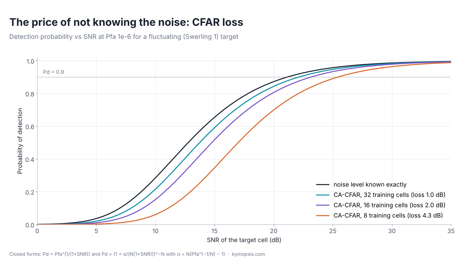
The other side is the probability of detection. A steady (non-fluctuating) target needs about 13 dB SNR in its cell to be detected 90 % of the time at P_fa = 10⁻⁶ (Albersheim’s approximation). A person is not a steady target: their echo fades and grows as they move, and for a target that fluctuates from frame to frame (the Swerling 1 model) the same 90 % needs about 21 dB. Where that SNR comes from, transmit power, antenna gain, range and integration, is the subject of the radar equation chapter.

Why a fixed threshold fails

In a quiet library a normal voice stands out; at a football match even a shout disappears. One fixed loudness line cannot work in both places, and a radar map has quiet places and loud places side by side.

σ² is not one number. In a real range-Doppler map the floor is higher at short range, where transmit-to-receive leakage and the cover’s own echo spill over; it rises around strong static objects, whose window sidelobes spread across neighbouring cells; it rises along the zero-Doppler line; and it changes with temperature and from unit to unit. A threshold that is right in the quiet part of the map produces a steady stream of false alarms in the busy parts. Set it for the busy parts, and weak targets in the quiet parts disappear.

CFAR: let the neighbours estimate the noise

You judge whether someone is shouting by comparing them with the people around them, not with silence. A CFAR detector does the same: each cell is compared with the average of its neighbours, so a target in a noisy patch has to stand out from that patch, and one in a quiet patch only from the quiet.

Constant false-alarm rate (CFAR) detection estimates σ² locally, for every cell, from the cells around it. Cell-averaging CFAR (CA-CFAR) takes N training cells in total, N/2 on each side of the cell under test, skips a few guard cells right next to it so the target’s own spread does not leak into the estimate, averages the training cells and multiplies by a factor α:

T = α · mean(training cells),    α = N · (P_fa^−1/N − 1)

Because the threshold scales with the local noise, the false-alarm rate stays the same wherever the floor goes, which is what the name promises. The price is that the noise estimate is itself noisy, so α must be larger than the known-noise factor to keep the same P_fa, and a slightly stronger target is needed for the same detection probability. That CFAR loss shrinks as the number of training cells grows:

More training cells mean a better noise estimate but a wider window, and a wide window is more likely to contain something that is not noise. Implementations commonly use somewhere between 4 and 16 training cells per side, fewer in Doppler, where the map is short.

When the neighbours are not noise

CA-CFAR fails in two common situations. Two targets close together put each other into their training cells, raise each other’s threshold, and the weaker one is masked (target B in the figure). And at a clutter edge, the training cells on one side sit in high clutter, the threshold jumps, and a target just inside the edge is lost while noise just outside it raises false alarms.

The standard fixes change how the training cells are combined. Ordered-statistic CFAR (OS-CFAR) sorts the training cells and uses, say, the 12th smallest of 16 instead of the mean, so one or two strong cells do not drag the threshold up; it costs a little more processing and a little more loss in clean noise. Greatest-of and smallest-of CFAR average each side separately and take the larger or smaller mean, which handles clutter edges or close targets respectively. Some processing chains use one variant in range and another in Doppler.

The formulas, and a check by simulation

With N training cells of exponential noise, their sum follows a gamma distribution, and the false-alarm probability of the test x > α·mean is (1 + α/N)^−N, which gives α = N(P_fa^−1/N − 1). For N = 16 and P_fa = 10⁻⁶ that is α = 21.9 (13.4 dB), against 13.8 (11.4 dB) with known noise. For a Swerling 1 target with SNR s, P_d = P_fa^1/(1+s) with known noise and P_d = (1 + α/(N(1+s)))^−N with CA-CFAR. A 400,000-trial simulation of the CA test at P_fa = 10⁻³ gives 1.09, 1.01 and 0.96 × 10⁻³ for N = 8, 16, 32. The steady-target figure of 13.1 dB is from Albersheim’s equation for a single look; integrating 16 looks non-coherently brings it to about 3.6 dB per look.

Clutter: echoes you do not want

To a radar a room is full of echoes: walls, a sofa, a table, a fridge, most of them stronger than you. The furniture gives exactly the same echo frame after frame, while a person’s echo flickers because people are never perfectly still. Average many frames, subtract the average, and what never changes disappears. Someone sitting very still fades too, which is why still-presence sensing needs the tricks in Chapter 11.

Clutter is everything that reflects but is not a target: walls, furniture, the floor, the housing. For an indoor radar it is usually far stronger than a person. The simplest and most effective tool against static clutter is to remove whatever does not change from chirp to chirp: subtract the mean of each range bin over the frame before the Doppler FFT, or high-pass the slow-time signal. Static echoes land exactly on zero Doppler and vanish; a walking person, whose phase moves from chirp to chirp, survives.

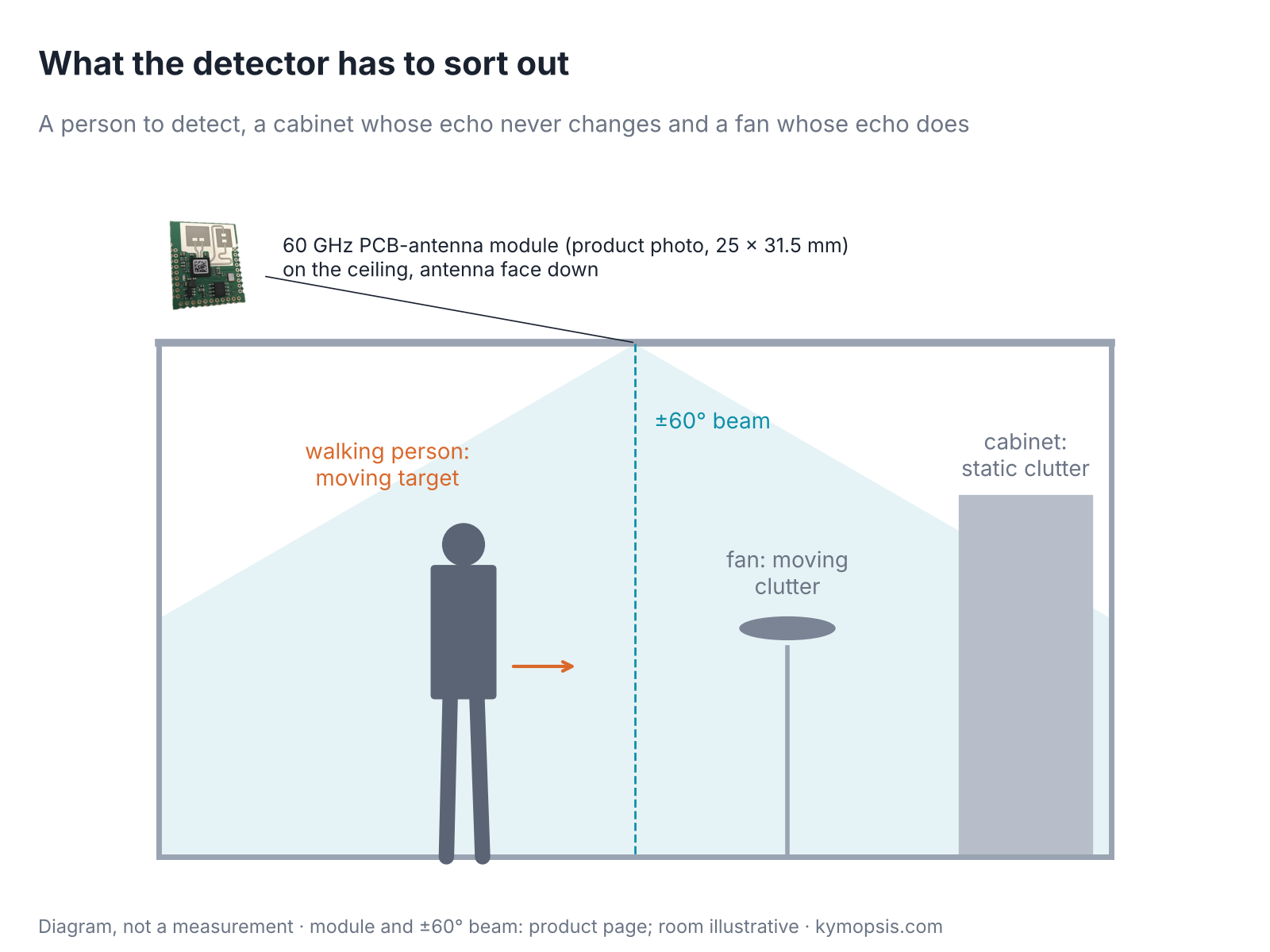
The catch is obvious once stated: a person sitting perfectly still is static clutter too. That is why presence sensors look for the much smaller motions of breathing and posture with longer observation windows, covered in the micro-Doppler chapter, and why ‘stationary presence’ is the hard specification in this product category. Moving clutter, such as fans, curtains in a draught or pets, is not removed this way and has to be handled by thresholds, region masks and tracking.

From detections to tracks

One footprint in the snow could be anything; a line of footprints, each where the last one said it would be, is clearly someone walking. A tracker trusts a detection only when it keeps turning up where the path predicts.

CFAR output is a list of cells per frame. One person produces several neighbouring cells, sometimes in more than one Doppler bin because arms and legs move differently. The first step is clustering: group detections that are close in range, velocity and angle into one object, often with a density-based method such as DBSCAN. Each cluster gets a position from its angle and range.

Those positions are still noisy, some frames miss the person, and a few false alarms survive. A tracker deals with all three. It keeps a state for each object, usually position and velocity, and runs a loop every frame:

1. Predict where each track should be now, from its last state and a motion model (constant velocity is the usual starting point), together with how uncertain that prediction is.
2. Gate: only detections inside an ellipse around the prediction, sized from that uncertainty, can belong to the track.
3. Associate and update: assign detections to tracks (nearest neighbour, or a global assignment when tracks are close), then blend each assigned detection into the state with a Kalman filter, weighting it by how much the measurement is trusted against the prediction.
4. Manage: start a tentative track from an unassigned detection, confirm it after M hits in N frames, and delete it after several misses. A track coasts on its prediction through short gaps.

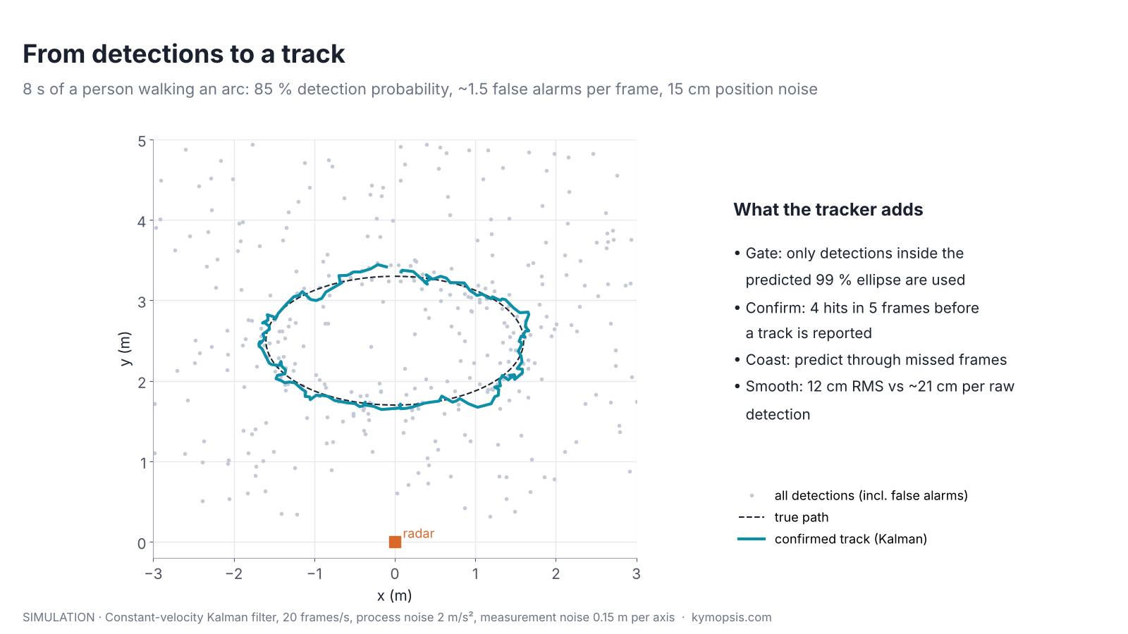
The confirmation rule is where false alarms really disappear. A random false alarm has to land inside a small gate four times in five frames to start a track, which is far rarer than one false alarm anywhere in the map. So the per-cell P_fa can be set looser than the product’s false-alarm budget, which recovers detection sensitivity. The price is latency: a 4-of-5 rule at 20 frames per second needs at least 200 ms before a new person appears in the output.

The Kalman filter in five lines

State x = [x, y, v_x, v_y], covariance P. Predict: x ← Fx, P ← FPFᵀ + Q, with F the constant-velocity transition over one frame and Q the process noise (how much the target may accelerate). Innovation: y = z − Hx, S = HPHᵀ + R, with R the measurement noise. Gate: accept z if yᵀS⁻¹y is below the chi-square threshold for two degrees of freedom (9.21 for 99 %). Update: K = PHᵀS⁻¹, x ← x + Ky, P ← (I − KH)P. Q is the main tuning knob: too small and the track lags when the person turns, too large and it follows the noise.

In a complete radar these steps sit in a fixed order with angle estimation between them: CFAR runs right after the range-Doppler FFT, angle is computed only at the detections, and the tracker takes the result. Chapter 21 follows that real-time chain end to end and counts what each step costs.

Detecting first is also what saves processing. Only one receive channel needs the full range-Doppler FFT for CFAR to run on. The other channels compute their complex value only at the detected cells, with a single-bin DFT that gives exactly the same number as a full FFT for a fraction of the work, and the angle is then read from the phase difference between the channels at those cells. Chapter 21 shows the single-bin DFT step by step, with the cost in multiplies, and chapter 12 how the phase difference becomes an angle.

Try it yourself: examples/ch16_cfar_tracking.py in the open-source radar-basics-sim repository runs the core simulation of this chapter; change the assumptions and see what moves.

What this means on the modules we sell

A sensitivity setting on a presence sensor is like the doorbell rule: turn it up and it notices a quieter, stiller person, but it also reacts more often to a fan or a moving curtain.

The presence firmware on our 60 GHz AiP and PCB-antenna development kits does its detection on the module and reports results over its serial interface. The maker does not publish the detector’s internals, so you do not tune α by hand, but the trade-offs above explain the behaviour you will see and what any sensitivity setting your firmware exposes is trading:

• A more sensitive setting means a lower effective threshold: weaker and more distant targets appear, and so do fans, curtains and reflections.
• Mounting close to a wall or behind a thick cover raises the near-range floor, so the first tens of centimetres are often masked or must be excluded.
• Someone who sits down and stops moving can drop out of a motion-based detector; stationary presence relies on micro-motion and longer hold times.
• If the output is tracked, reported positions are smoothed, so they lag a quick movement slightly. That lag is the cost of steadier output.

The open-source Radar Desk Buddy reads the target reported by the AiP module and turns a servo to follow it, which makes the confirmation delay and smoothing easy to see. The firmware’s internal parameters are not published by the module maker, so we describe its behaviour, not its numbers.

GitHub · Kymopsis /radar-desk-buddyESP32-S3 desk companion with a 60 GHz mmWave radar: eyes and figure follow you, local time and weather, Telegram messages. No soldering.CMIT licenseView repository → GitHub · Kymopsis /radar-basics-simView repository → B2B engineering · KymopsisFalse alarms or missed targets in your application?Describe the room, mounting and what must be detected. We scope radar modules, placement and processing for B2B projects.Describe your scene

FAQ

What is CFAR in radar?

Constant false-alarm rate detection: each cell’s threshold is set from the average (or a ranked value) of the cells around it, multiplied by a factor chosen for the wanted false-alarm probability. The false-alarm rate stays constant even when the noise and clutter level changes across the map.

Why does my radar see targets where nothing is moving?

Common causes are moving clutter (fans, curtains, plants in a draught), multipath reflections of a real person off walls or the ceiling, and a sensitivity set so high that noise crosses the threshold. Tracking confirmation and region masks remove most of them.

Why does a person who sits still disappear?

Static-clutter removal treats anything that does not change from chirp to chirp as background. A still person only moves by breathing, a few millimetres, which needs longer observation and dedicated micro-motion processing to detect.

Does a Kalman filter improve detection?

It does not find targets the detector missed, but it bridges short gaps, rejects isolated false alarms through gating and confirmation, and reduces position noise. The confirmation logic also allows a looser per-cell threshold, which indirectly improves sensitivity.

Sources and method

• M. A. Richards, Fundamentals of Radar Signal Processing, 2nd ed., McGraw-Hill, 2014: CFAR detection and CFAR loss.
• M. A. Richards, J. A. Scheer, W. A. Holm (eds.), Principles of Modern Radar: Basic Principles, SciTech, 2010: detection fundamentals and Swerling models.
• W. J. Albersheim, ‘A closed-form approximation to Robertson’s detection characteristics’, Proc. IEEE, vol. 69, no. 7, 1981.
• Y. Bar-Shalom, X. R. Li, T. Kirubarajan, Estimation with Applications to Tracking and Navigation, Wiley, 2001: Kalman filtering, gating and track management.
• MIT OpenCourseWare, Introduction to Radar Systems (Lincoln Laboratory), detection lectures (ocw.mit.edu).

All figures are computed from the closed forms or simulated with the Kymopsis Radar Principles scripts (ch16_cfar_tracking.py): exponential noise, CA/OS-CFAR with 8 training and 2 guard cells per side, a constant-velocity Kalman filter at 20 frames/s. None is measured data from the modules we sell.