Radar Principles 3: Interference, Multipath and Ghost Targets

Point a 60 GHz radar at a person standing still in a room and the echo strength is not one number. Move the person two centimetres and it can drop by 20 dB, then come back. Nothing is wrong with the radar: the echo is reaching it along several paths, and the paths add up or cancel depending on their phase. The same effect lets an antenna array form a beam, makes a radome act like a mirror at the wrong thickness, and puts false targets in a tank. This chapter is about adding waves.

Superposition: waves add as arrows

Drop two pebbles into a pond and watch where their rings cross. Where a crest meets a crest, the water jumps twice as high; where a crest meets a trough, the water stays almost flat. Noise-cancelling headphones use the same trick with sound: they add a copy of the noise turned upside down, and the two cancel. Radio waves add exactly like this, and a radar’s echo is often several waves arriving together.

Electromagnetic fields obey the superposition principle: when two waves overlap, the total field at each point is simply the sum of the two fields. Because each wave is a rotating arrow (the phasor from chapter 2), “sum” means adding arrows tip to tail. Two waves of equal frequency make a third wave of the same frequency whose amplitude depends on how far apart in phase the two arrows point.

• In phase (0°): the arrows line up and the amplitudes add, 1 + 0.8 = 1.8. Constructive interference.
• In opposition (180°): they point opposite ways and subtract, 1 − 0.8 = 0.2. Destructive interference.
• Anything in between: the amplitude is √(a₁² + a₂² + 2a₁a₂·cos Δφ).

Note that it is the fields that add, not the powers. 1.8² is 3.24 and 0.2² is 0.04: a factor of 81, or 19 dB, between the best and worst case, caused only by a change in phase. A phase change of 180° at 60 GHz takes a path difference of 2.48 mm, or a target movement of 1.24 mm if the path difference is a round trip. That is why the effects below are so sensitive to position.

Two sources make a pattern

Drop the two pebbles at the same moment, a little apart, and the crossing rings settle into spokes: lines of rough water running outward, with calm lines between them. Stand on the bank in one direction and you see big waves; walk a few steps along the bank and the water in front of you is still. Two antennas fed with the same signal paint the same spokes into space.

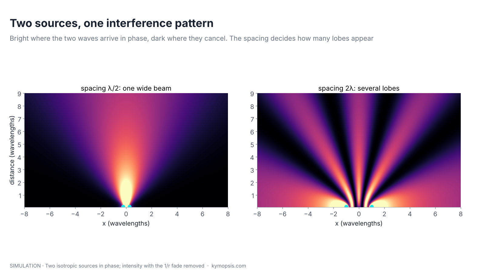
Put two small antennas side by side, a distance d apart, and drive them with the same signal. A point far away at angle θ from straight ahead sees the two waves arrive with a path difference of d·sin θ, which is a phase difference of 2π·d·sin θ/λ. Wherever that phase difference is a whole number of turns, the waves add (a lobe); wherever it is half a turn off, they cancel (a null). The figure at the top shows the result.

• At d = λ/2 the phase difference can never reach a full turn away from broadside, so there is one broad lobe facing forward.
• At d = 2λ it passes through several full turns as θ sweeps from −90° to +90°, so several equally strong lobes appear, with nulls between them.

This one picture explains three later chapters. Receive antennas spaced λ/2 apart can tell angles apart without confusion (chapter 12). Spacing them further apart makes extra lobes, the grating lobes that create angle ambiguity (chapter 15). And many antennas in a row make one very narrow lobe, which is how arrays get their resolution (chapter 17).

Steering the pattern with phase

Now drop one pebble a moment after the other. The spokes of rough water swing to one side, although neither pebble moved. A radar does this electronically: delay one antenna’s signal a tiny fraction of a cycle and the strong direction turns.

If one of the two sources is fed with an extra phase shift, the condition for adding in phase moves to a different angle: the lobes turn. Nothing moves mechanically.

A lobe forms where 2π·d·sin θ/λ + Δφ_feed = 0, so sin θ = −Δφ_feed·λ/(2πd). With more than two elements and a controlled phase on each, this becomes a phased array: chapter 17 covers it, with the practical limits.

Standing waves

A microwave oven has hot and cold spots, which is why it turns the plate. The wave bounces back and forth between the metal walls and the outgoing and returning waves add into peaks that stay in place, about 6 cm apart at 2.45 GHz. At 60 GHz the same peaks are only 2.5 mm apart, so a radome a fraction of a millimetre too thick or too thin can sit on a peak or a null.

When a wave meets a surface head-on and part of it reflects, the outgoing and returning waves overlap in the same space. Their sum no longer travels; it forms fixed peaks and nulls half a wavelength apart, a standing wave. The two places where radar engineers meet this every day are:

• The radome. A plastic cover reflects a little at its front face and a little at its back face. If the two reflections are in opposition they cancel and the cover is almost transparent; if they are in phase the cover acts like a mirror and blinds the radar. The thickness that cancels is a multiple of half a wavelength inside the plastic. Chapter 13 works through it.
• Leakage close to the antenna. Energy bouncing between the antenna and a nearby cover or housing creates a strong signal at very short range, which hides targets in the first few centimetres.

Multipath fading

Most people have met this with Wi-Fi or a phone: one spot on the sofa has no signal, and moving a hand’s width fixes it. The signal arrives directly and off a wall or floor, and in the dead spot the two cancel. A 60 GHz radar sees the same thing with its waves 25 times shorter than Wi-Fi’s, so the dead spots are only a few centimetres apart.

Outside the lab, the radar’s signal reaches a target along more than one path. The classic case is a radar mounted above a floor or road: one path goes straight to the target, the other bounces off the floor. The two arrive with a path difference Δ that changes with the target’s distance and height, so their sum goes through peaks and nulls.

For a radar the effect is applied twice, once on the way out and once on the way back, so the echo power varies as |1 + Γ·e^−jkΔ|⁴, where Γ is the floor’s reflection coefficient. With Γ = −0.7 the echo swings between +9 dB and −21 dB compared with free space. At 60 GHz the nulls are only a few centimetres apart at room distances, and moving the target 2 cm up or down shifts them completely.

Where the formula comes from

With radar height h_r, target height h_t and horizontal distance d, the direct path is √(d² + (h_r − h_t)²) and the floor-bounce path is √(d² + (h_r + h_t)²). Their difference Δ is approximately 2h_rh_t/d for d much larger than the heights. One way, the field is multiplied by F = |1 + Γe^−j2πΔ/λ|; two ways, the power by F⁴. Nulls occur when 2πΔ/λ makes the two terms opposite, and their spacing in distance is about λd²/(2h_rh_t), about 3 cm at 3.5 m for the numbers in the figure.

Three things soften this in practice. Real antennas have a beam, so the floor path is weaker than the direct one when the radar is tilted slightly upwards. Real floors are rough and reflect less coherently. And a wide-band FMCW radar sees the two paths at slightly different ranges: when the path difference exceeds the range resolution, they fall into different range bins instead of cancelling (chapter 6).

Ghost targets

Shout towards a cliff and you hear your voice come back later, as if someone further away were answering. Look into a mirror and a second room appears behind the glass. A radar is fooled the same way: an echo that came back by a detour through a wall looks like a second target standing further away.

When the extra path is long enough to be resolved, multipath stops being fading and starts being a false target. A radar measures the total path length and divides by two, so:

• a path that goes radar → wall → target → radar appears at half the sum of the two legs, slightly behind the real target and often at a different angle;
• a double bounce, radar → target → radar housing → target → radar, appears at twice the range of the real target.

Both are common in practice. In a tank, a level radar sees the liquid surface, but also the tank wall, agitator blades, ladders and the double bounce between surface and tank roof. Level radars therefore commonly record an echo map of the empty or partly filled tank and suppress echoes that stay at fixed ranges. In rooms, a person near a metal cabinet can appear twice in a presence radar’s point cloud. Tracking (chapter 16) and angle checks help separate the real target from its mirror image.

Many scatterers in one cell

Sunlight on a lake glitters, and the sparkles change as the water moves even slightly, because each sparkle is light from many tiny tilted patches adding up. A person or a car is the same for a radar: many small reflecting patches, so a slight turn can make the echo jump up or down even though the distance has not changed.

A person, a car or a heap of grain is not one reflector but many, all inside the same range bin. Their echoes add as arrows too. When the object turns slightly, the arrows rearrange and the total amplitude fluctuates, sometimes by 10 dB or more, even though the object is the same distance away. This is why radar cross-section is described statistically, and why detection needs a margin above the average echo. Chapter 7 puts numbers on that margin.

What this means for real installations

• Do not judge a mounting position by one static reading. Move the target a few centimetres and watch the spread of readings.
• Tilting a presence or ranging radar a few degrees away from a floor or ceiling often removes the strongest multipath path.
• Keep reflective objects out of the beam close to the radar, and choose a cover thickness that the wave passes cleanly (see radomes).
• For tanks, mount the gauge away from the wall and from the inlet stream; the antenna article in chapter 4 compares beam widths.

All figures here come from the open-source radar-basics-sim library; the two-ray model and the ghost profile can be rerun with your own heights, distances and reflection coefficients.

Try it yourself: examples/ch03_multipath.py in the open-source radar-basics-sim repository runs the core simulation of this chapter; change the assumptions and see what moves.

GitHub · Kymopsis /radar-basics-simView repository → B2B engineering · KymopsisNeed this built into your product?Custom radar modules, antennas and enclosures, from prototype to volume. Send your requirements and we reply with options and a quote.Request a quote →

FAQ

Why does my radar’s signal strength jump when I move the target slightly?

Because the echo arrives along several paths whose phases change with position. At 60 GHz a few millimetres is enough to move from a peak to a null of the multipath pattern.

Is interference the same as multipath?

Multipath is one cause of interference: the same signal arriving over different paths. “Interference” is also used for signals from other radars, which is a different problem.

Can a wider bandwidth remove multipath?

It helps. When the path difference is larger than the range resolution (about 3.75 cm for a 4 GHz sweep), the paths fall into different range bins and stop cancelling. The longer path then shows up as a separate, weaker target.

Why do antenna arrays use half-wavelength spacing?

It is the widest spacing that still forms a single main lobe across the whole forward half-space. Wider spacing gives a narrower beam but adds grating lobes.

Sources and method

• C. A. Balanis, Antenna Theory: Analysis and Design, 4th ed., Wiley, 2016 (two-element arrays, array factor).
• M. I. Skolnik, Introduction to Radar Systems, 3rd ed., McGraw-Hill, 2001 (multipath and the propagation factor).
• M. A. Richards, Fundamentals of Radar Signal Processing, 2nd ed., McGraw-Hill, 2014 (target fluctuation).
• Figures and animations are computed in Python from the formulas shown; the simulation code is open source in Kymopsis/radar-basics-sim. Figures marked SIMULATION are not measurements of a product.