


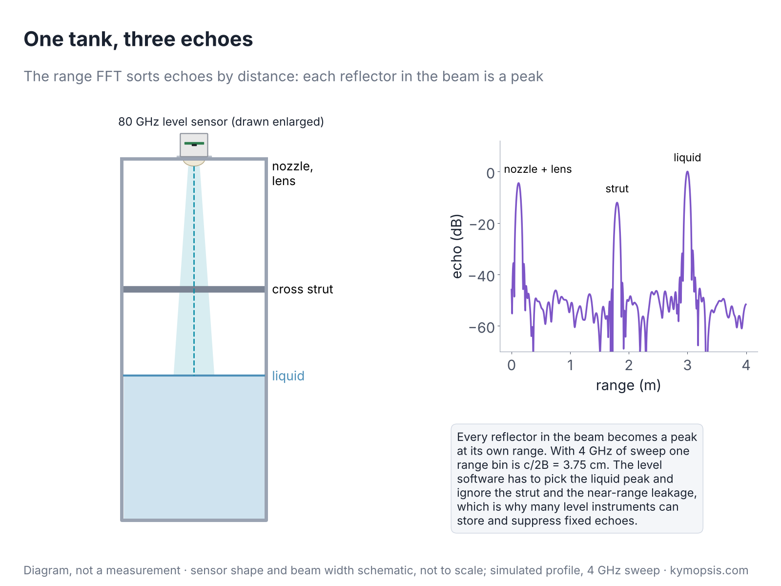
Point an 80 GHz level sensor down into a tank and three things answer: the nozzle it is mounted in, a cross strut halfway down, and the liquid surface. They come back as one beat signal, a sum of three tones that looks like noise. The task of this chapter is to pull them apart into three peaks at three distances.
The beat signal from chapter 5 becomes useful only after a Fourier transform turns it into a range profile: echo strength against distance. That one step decides how close two targets can be and still appear as two, how a weak target next to a strong one survives, and how finely the radar’s distance axis is divided. This chapter takes the range FFT apart, including two points that confuse many people: why zero padding does not improve resolution, and why the resolution is not the precision.
Time and frequency: two views of one signal
A piece of music can be drawn as one wiggly line on an oscilloscope, or as the bouncing bars of a music player’s equaliser, one bar for each pitch. Both pictures show the same sound. The Fourier transform turns the first picture into the second, and a radar reads distance from the second.
Before taking the range FFT apart, it helps to be clear about what a Fourier transform does, because everything in the rest of this series leans on it. Any recorded signal can be described in two equivalent ways. In the time domain it is a list of values, one per sample, which is what the ADC delivers. In the frequency domain it is a list of tones, each with an amplitude and a phase, that add up to the same signal. The Fourier transform converts the first description into the second without losing anything, and the inverse transform converts back.

Three rules from the figure are worth remembering, because the rest of the chapter is built on them:
- A steady tone becomes a single peak. Its position is the tone’s frequency. For a radar, one target gives one beat tone (chapter 5), so one target gives one peak, and the position is the range.
- A shorter record gives a wider peak. Recording a tone for a time T smears its peak over about 1/T in frequency. This is not a flaw of the FFT; a short piece of signal simply does not contain enough cycles to pin the frequency down. It is the reason range resolution depends on how long, in swept bandwidth, the radar listens.
- A sum of tones becomes a set of peaks. In time, two targets give a messy-looking signal; in frequency they are two separate peaks. Several targets, clutter and noise all add in the time domain and stay apart in the frequency domain, which is why radars process in frequency.
How does the FFT find the tones? Each of its outputs answers one question: how much of this particular frequency is in the signal? It multiplies the samples by a test tone of that frequency and averages the product. If the signal contains the test tone, the two rise and fall together, the product is mostly positive and the average is large. If not, the product swings positive and negative and averages to almost nothing.
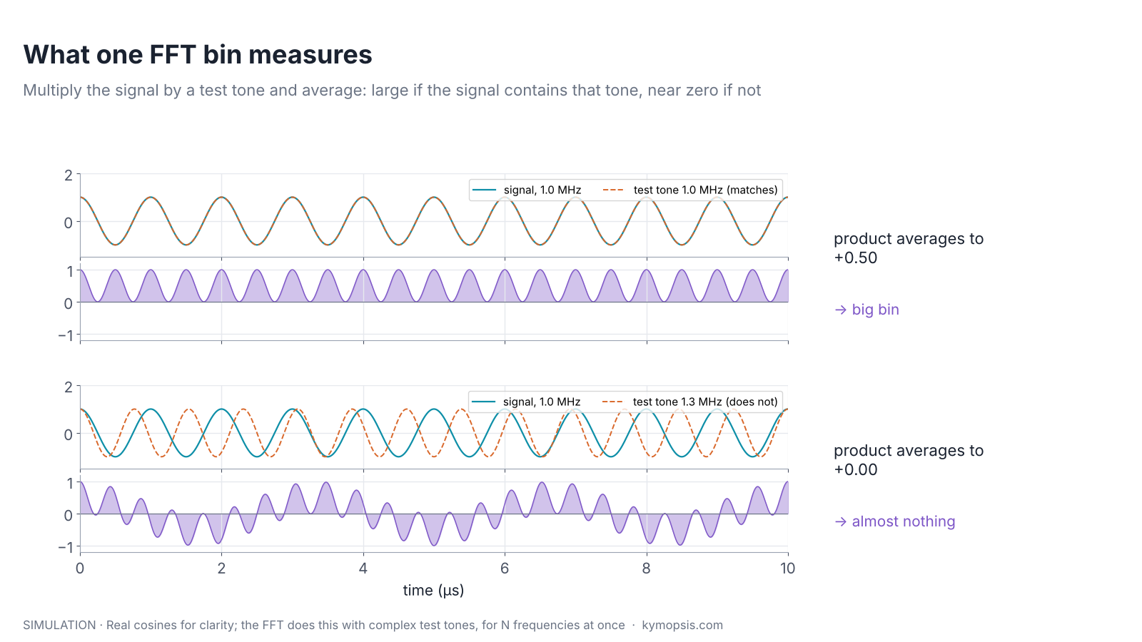
A discrete Fourier transform (DFT) does this for N test tones, evenly spaced, and the FFT is simply a fast way of computing all N at once. It uses complex test tones (cosine and sine together, as in chapter 2), so that each output also carries the phase of the matching tone, not only its strength.
The DFT formula, and why the test tones are spaced 1/T apart
For samples x[n], n = 0…N−1, output k is X[k] = Σ x[n]·e−j2πkn/N. The factor e−j2πkn/N is the complex test tone at frequency k·fs/N. Neighbouring test tones differ by fs/N = 1/T, where T = N/fs is the record length: over the record they differ by exactly one full cycle, so a tone sitting exactly on one of them averages to zero against every other one. That spacing is the frequency resolution 1/T from rule 2, and in range it becomes c/2B.
From samples to range bins
Think of a row of numbered pigeonholes, one for every few centimetres of distance. The FFT sorts the beat signal into such a row, and each echo lands in the pigeonhole for its range.
During one chirp the ADC records N samples of the beat signal at rate fs. An N-point FFT turns them into N complex values. Value k holds the part of the signal near frequency k·fs/N, and since beat frequency is proportional to range, each FFT output is a range bin:
Rk = k · c / (2Bs), where Bs = S·N/fs is the bandwidth swept while the ADC was recording.
Each bin is a complex number, even when the ADC recorded only a real signal: with real samples the upper half of the outputs mirrors the lower half, so only the first N/2 are used as range bins, but each still has an amplitude and a phase. Why a real signal still gives complex bins, and what complex (I/Q) sampling changes, is worked through in Radar Math 1. Its magnitude says how much echo came from that distance; its phase is the echo phase from chapter 2, which later chapters use for Doppler, angle and micro-motion. The magnitude in decibels, plotted against Rk, is the range profile.
Why the resolution is c/2B
Two people stand side by side in front of a radar, and it counts one. Each echo in the range spectrum is not a thin line but a small hill, and the width of that hill is set by how wide the chirp sweeps. A 4 GHz sweep gives hills under 4 cm wide, so two people 10 cm apart in range show up as two peaks; narrow the sweep to 1 GHz and the hills grow to 15 cm and melt into one. Direction (Chapter 12) and speed (Chapter 10) are the other two ways a radar can pull them apart again.
An FFT over a record of length T can only tell apart frequencies that differ by about 1/T: two tones closer than that do not complete enough relative cycles within the record to separate. The record length is N/fs and the beat frequency per metre is 2S/c, so the smallest separable range difference is
ΔR = (1/T) · c / (2S) = c / (2 · S · T) = c / (2B)
The slope cancels out. Only the bandwidth swept during the sampling window counts: a slow, wide chirp and a fast, wide chirp have the same resolution.
| Swept bandwidth | Range resolution c/2B | Where you meet it |
|---|---|---|
| 250 MHz | 60 cm | 24 GHz ISM band (24.0–24.25 GHz) |
| 1 GHz | 15 cm | Narrow-band 60 GHz or 80 GHz settings |
| 4 GHz | 3.75 cm | 76–81 GHz and many 60 GHz configurations |
| 7 GHz | 2.1 cm | Full 57–64 GHz band, where regulations allow |
Which bandwidth a radar may sweep depends on the band’s radio rules, which is a large part of the comparison in chapter 20.
When two targets merge
A car’s two headlights far down a dark road look like one light; as the car comes closer, they split into two. Two radar echoes behave the same way: when their ranges are too close, their hills melt into one.
ΔR is a rule of thumb, not a hard edge. Watching two equal targets approach each other shows three things:
- Around one to two bins apart the dip between the peaks fades and the two targets become one. The exact point depends on the window and on the two echoes’ relative phase; the animation keeps them in phase, and out-of-phase echoes separate a little earlier.
- Before they merge, the peaks are pulled or pushed away from the true positions (the dashed lines). Close targets bias each other’s range readings.
- A wider main lobe, from the Hann window, merges earlier than the rectangular window.
This is why a radar with 3.75 cm resolution can still see a person and the chair they sit on as one blob: body and chair are a few centimetres apart in range. Angle (chapter 12) and velocity (chapter 10) give other dimensions in which they may separate.
Windows and side lobes
A bright street lamp seen through a camera lens has a halo, and a dim star beside it vanishes in the glow. A strong echo makes a similar halo, its side lobes. A window dims the halo so the faint neighbour shows, at the price of a slightly wider spot.
Taking N samples and stopping is the same as multiplying an endless signal by a rectangle. In the frequency domain the rectangle becomes a sinc shape: a main lobe with a long tail of side lobes, the first only 13 dB below the peak. A strong target therefore spreads energy over the whole profile, and a weak target nearby can drown in it, as the figure below shows.

A window tapers the samples smoothly to zero at both ends before the FFT. The edges of the record stop being abrupt, and the side lobes fall dramatically. The price is a wider main lobe (coarser effective resolution) and a small loss in SNR, because the tapered samples carry less of the echo energy.
| Window | First side lobe | Main lobe width (null to null) | SNR loss |
|---|---|---|---|
| Rectangular | −13 dB | 2 bins | 0 dB |
| Hann | −31 dB | 4 bins | ≈1.8 dB |
| Blackman | −58 dB | 6 bins | ≈2.4 dB |
Most radar firmware uses a Hann or similar window on the range FFT. Level gauges, which must find a liquid surface next to strong echoes from tank fittings, often go further toward low-side-lobe windows.
Where the SNR loss comes from
A window w[n] scales the echo, which adds coherently, by Σw/N, and the noise, which adds in power, by √(Σw²/N). The ratio gives the equivalent noise bandwidth, ENBW = N·Σw²/(Σw)², in bins: 1 for rectangular, 1.5 for Hann, about 1.73 for Blackman. The SNR loss is 10·log10(ENBW): 0, 1.76 and 2.37 dB.
Zero padding
Zooming into a blurry photo makes it bigger, not sharper. Zero padding is that zoom: a smoother drawing of the same spectrum, with no new detail in it.
Appending zeros to the samples before the FFT gives more output points, so the profile is drawn on a finer grid. It is tempting to think that this improves resolution. It does not: the information in the record is unchanged, and the main lobe keeps its width.
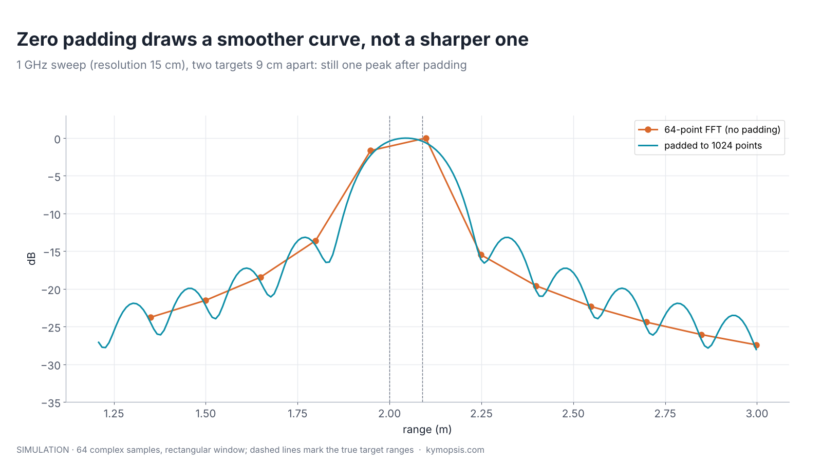
What zero padding does do is useful: it reveals the true peak position between the original bins, which a coarse grid can miss by up to half a bin, and it recovers some of the peak height lost when the target sits between two bins (the scalloping loss, up to 3.9 dB for a rectangular window). That is the start of the subject of chapter 8.
Resolution is not precision
A blurry photo may not show whether one or two people stand in the doorway, yet you can still point to the exact middle of the blur. Resolution is telling the two apart; precision is pointing to the middle.
Resolution answers “can I tell two targets apart?” Precision answers “where exactly is this one target?”. For a single strong target, the second can be far finer than the first. A level gauge with a few centimetres of range resolution reports a liquid level to millimetres, because the peak’s exact position can be estimated from the shape of the main lobe, and that estimate improves with SNR. Chapter 8 shows how, and chapter 9 goes another thousand times finer with phase.
Phase noise and range correlation
A singer whose pitch wobbles slightly blurs every note. A radar’s oscillator wobbles too, but the echo and the reference it is compared with wobble almost together, so a near echo barely notices; only far echoes, which come back from an older moment, see the blur.
Windows control the skirt that the FFT itself puts around a strong peak. A second skirt comes from the oscillator. No real synthesiser produces a perfect chirp: its phase wanders by small random amounts, and that phase noise appears in a spectrum as a skirt of power on both sides of every tone. Datasheets quote it as L(f) in dBc/Hz: the noise power in 1 Hz at an offset f from the carrier, relative to the carrier.
An FMCW radar is far more tolerant of phase noise than this number suggests, because the mixer compares the echo with the same oscillator a moment later. If the echo’s delay τ = 2R/c is short, the transmitter has hardly had time to wander, the two copies carry almost the same phase error, and the multiplication in the mixer (chapter 5) cancels it. This is range correlation. What survives is the phase-noise spectrum multiplied by 4·sin²(πfτ), which is tiny when fτ is small and grows with range.

The figure uses an illustrative synthesiser (−85 dBc/Hz inside a 300 kHz loop, falling 20 dB per decade outside) with a 100 MHz/µs slope and 25 kHz range bins, so 1 MHz of offset is 1.5 m of range. At that offset the cancellation is 53.6 dB for a reflector at 5 cm, 18.0 dB at 3 m and only 8.5 dB at 9 m. The practical consequences follow directly:
- Leakage and radome echoes, the strongest signals in most profiles, sit within centimetres of the antenna and add almost no phase-noise skirt. Their own peak and window side lobes matter far more.
- A strong far reflector, such as a wall, a metal shelf or the tank bottom, carries a skirt that is only partly cancelled. It lifts the noise floor for several metres around it and can hide a weak target there, such as a person standing next to a wall, even when the window is good.
- Short-range sensors (gesture, presence, level gauges over a few metres) can therefore use fairly ordinary synthesisers. Long-range automotive radar, where a weak pedestrian sits near a strong truck 100 m away, is where phase noise becomes a headline specification.
The numbers above describe the model, not any particular chip. For a real module, take L(f) from the radar chip’s datasheet and apply the same factor.
Deriving the 4·sin²(πfτ) factor
Write the transmitted phase as 2π·(f0t + St²/2) + φ(t), where φ(t) is the random phase noise. The echo is the same signal delayed by τ. The mixer output keeps the phase difference, which contains φ(t) − φ(t − τ). Delaying a signal by τ multiplies its spectrum by e−j2πfτ, so the difference has spectrum Φ(f)·(1 − e−j2πfτ). Its power is |1 − e−j2πfτ|² = 2 − 2cos(2πfτ) = 4·sin²(πfτ) times the original. For small fτ this is about (2πfτ)², a 20 dB-per-decade rise with both offset and range. At 5 cm, τ = 0.33 ns, and at 1 MHz offset 4·sin²(πfτ) = 4.4×10⁻⁶, or −53.6 dB.
The skirt level in a range bin is L(f) + 10·log10(bin width) + 10·log10(4·sin²(πfτ)). With −85 dBc/Hz flat to 300 kHz then −20 dB/decade, L(1 MHz) ≈ −95.8 dBc/Hz; a 25 kHz bin adds 44 dB, giving −51.9 dBc uncorrelated and −105.4, −69.9 and −60.4 dBc for reflectors at 0.05, 3 and 9 m.
A range FFT in five lines
import numpy as np
c, B = 299792458, 4e9                       # swept bandwidth during sampling, Hz
w = np.hanning(adc.shape[-1])                # adc: real or complex samples [chirps, rx, samples]; with real samples keep the first half of the bins
profile = np.fft.fft(adc * w, axis=-1) / w.sum()
ranges = np.arange(adc.shape[-1]) * c / (2 * B)   # metres per bin
The open-source radar-basics-sim library wraps this as range_fft(), and its range-resolution example reproduces the animation above with your own target spacing and window.
What a real range profile looks like
A real profile has more in it than the simulations: a strong peak near zero from transmitter leakage and the radome, the target, its multipath ghosts from chapter 3, and a noise floor that rises near strong echoes, partly from the window and partly from phase noise. Reading one is a matter of asking, for each peak, what in the scene could produce it: a peak that stays put when the target moves is a fixed reflector or leakage; a peak at exactly twice a strong target’s range is usually a double bounce; and a wide hump around a strong far reflector is its skirt, not a group of targets. Level gauges add a step in software: they record an empty-tank profile once and subtract or mask the fixed echoes from nozzles, ladders and welds, so the surface echo is the only peak left to track. The antenna and lens choices that shape the curve are covered in chapter 4.
A profile is only as clean as the beat signal that went into the FFT. Tones above the ADC’s limit fold back as false peaks at short range, which is why the IF low-pass in front of the ADC matters. On a bench, when the IF is brought out on coax to an oscilloscope or a separate ADC, an in-line coaxial low-pass filter does the same anti-alias job. Its cutoff must sit below half the sampling rate, so a DC–50 MHz filter suits sampling at 100 MS/s or faster.
Try it yourself: examples/ch06_range_resolution.py in the open-source radar-basics-sim repository runs the core simulation of this chapter; change the assumptions and see what moves.
-

80 GHz Radar Level Sensor Development Kit, 76–81 GHz, 20 or 60 Meter Range
From $99.00Reset options60-meter kit, horn + lens20-meter kit, lens radomeSelect options This product has multiple variants. The options may be chosen on the product page
FAQ
What does an FFT do to a radar signal?
It converts the sampled beat signal from the time domain into the frequency domain: a list of tones with their strengths and phases. Each target’s beat tone becomes one peak, and the peak’s position is the target’s range.
Does a higher frequency radar have better range resolution?
Not directly. Resolution is c/2B and depends only on swept bandwidth. Higher bands simply allow wider sweeps: 4 GHz at 77–81 GHz against 250 MHz at 24 GHz.
Can I get better resolution by sampling faster?
No. Faster sampling extends the maximum range for the same slope, but resolution stays c/2B. More samples over the same sweep only add bins at longer range.
Why do my two targets show three peaks?
Usually side lobes or multipath. Try a Hann window and check whether the extra peak moves with one of the targets.
What is a range bin in a radar datasheet?
The spacing of the range profile, normally c/2B. Some datasheets quote it as “distance resolution” and quote a separate, finer “accuracy”.
Sources and method
- F. J. Harris, “On the use of windows for harmonic analysis with the discrete Fourier transform”, Proc. IEEE, 1978 (window figures).
- M. A. Richards, Fundamentals of Radar Signal Processing, 2nd ed., McGraw-Hill, 2014 (range resolution, straddle loss).
- Texas Instruments, Introduction to mmWave Sensing: FMCW Radars, training series (concepts).
- Figures and animations are computed in Python from the formulas shown; the simulation code is open source in Kymopsis/radar-basics-sim. Figures marked SIMULATION are not measurements of a product.