



A radar with 3.75 cm range bins can report a distance to a fraction of a millimetre. That sounds like a contradiction until you separate two questions. Resolution, from chapter 6, is about telling two targets apart. Precision is about locating one target, and for a single clean echo it is limited by noise, not by the bin size. This chapter shows how a radar reads range between the bins, how good that reading can get, and what stops it in practice.
The peak sits between the bins
A thermometer is marked every degree, but the liquid stops wherever the temperature is, usually between two marks. Reading only the nearest mark throws away where it really stopped. A range FFT has the same marks, its bins, and the echo almost always sits between two of them.
An FFT samples the range profile at fixed points, the bin centres. A real target is almost never exactly on one. If it lies 40% of the way from bin 40 to bin 41, the main lobe straddles the two and both bins show part of the echo. Picking the strongest bin rounds the range to the nearest bin centre: an error that is uniformly spread between −½ and +½ bin, i.e. ±18.75 mm for 3.75 cm bins, or about 10.8 mm RMS.
But the shape of the main lobe is known exactly: it is the Fourier transform of the window. The heights of the strongest bin and its two neighbours therefore say where the true peak is. That is the whole idea.
Interpolating the peak
A hiker who knows the height at three points along a ridge can sketch a smooth hump through them and say where the summit lies, even if it falls between the points. Peak interpolation does exactly that with the three tallest bins.

Three practical methods, in rising order of cost:
- Parabolic interpolation. Fit a parabola through the peak bin and its two neighbours and take its vertex. With magnitudes α, β, γ the offset in bins is δ = ½(α − γ)/(α − 2β + γ). Fitting the parabola to the logarithm of the magnitudes works much better for Hann-type windows, because their main lobe is close to a Gaussian, whose logarithm is exactly a parabola. In the figure: under 2 mm of bias on magnitude, under 0.6 mm on log magnitude.
- Zero padding plus interpolation. Pad the FFT (chapter 6) so that the grid is already fine, then interpolate. The remaining bias drops to the micrometre level.
- Zoom FFT or iterative fitting. Evaluate the spectrum only around the peak on a very fine grid (chirp-z transform), or fit the exact lobe shape by least squares. These reach the theoretical limit and are used where every micrometre counts.
Why the logarithm helps
A Gaussian e−a(k−k₀)² becomes −a(k−k₀)² after taking the logarithm: a parabola with its vertex exactly at k₀, so three points determine it without error. A Hann window’s main lobe is not exactly Gaussian, which leaves the small residual bias in the figure. For a rectangular window, the magnitude near the peak is a sinc and other closed-form estimators (Jacobsen’s or Quinn’s, which use the complex bin values) work better.
The precision limit
Try to point at the middle of a lamp seen through mist: in thin mist your guesses cluster tightly, in thick mist they scatter. Noise is the mist, and for each amount of it there is a tightest cluster that no method can beat.
With noise, every estimate scatters. Estimation theory gives a floor for that scatter, the Cramér–Rao lower bound. For the frequency of a single tone in white noise it gives, expressed in range bins,
σk ≥ √6 / (2π · √SNR), so σR ≥ ΔR · √6 / (2π · √SNR)
where SNR is the signal-to-noise ratio after the range FFT (chapter 7). Every 10 dB of SNR makes the error about 3.2 times smaller. At 40 dB with 3.75 cm bins the bound is 0.15 mm; at 60 dB, 15 µm.
The Monte Carlo result at the top of the page compares real estimators with this bound. Three regions are visible:
- Low SNR (below about 15 dB): noise sometimes wins and the wrong bin is chosen, so the error jumps to whole bins. This is the threshold effect. Detection must be reliable before precision means anything.
- Middle: the padded estimator stays within about 1.5 times the bound, the plain log-parabola within about 2 times. The window costs part of that gap, because it lowers the SNR slightly.
- High SNR: the plain log-parabola levels off at its own bias of a few tenths of a millimetre, while the padded version keeps improving. At high SNR, the estimator’s systematic error, not noise, is the limit.
Watching it work
At 35 dB the interpolated reading follows the target with a scatter of well under a millimetre while the bin reading sits still and then jumps by a full bin. Every radar that reports a smooth distance does some version of this.
What limits it in practice
A bathroom scale that reads two kilograms too heavy gives the same wrong answer every morning, and weighing yourself a hundred times does not fix it. Multipath, offsets and drift are errors of that kind, and averaging does not remove them.
The bound assumes one target, white noise and a perfect radar. Real measurements add systematic errors that averaging does not remove:
- Neighbouring echoes. A second reflector within a few bins distorts the main lobe and pulls the estimate, the bias visible in chapter 6‘s merging animation. Multipath (chapter 3) is the most common source.
- Chirp non-linearity. A curved ramp broadens and shifts the peak by an amount that can depend on range.
- Reference offset. Cables, antenna feed and radome add a fixed delay. It is calibrated with a target at a known distance.
- Temperature drift. The synthesiser’s slope and the electronics’ delay change slightly with temperature; precise instruments compensate for it.
- Target shape. For a person or a heap of material the “range” is an average over many scatterers and is not well defined below the centimetre level.
How level radars reach millimetres
A carpenter gets the most exact measurement on a long, straight board with nothing in the way and time to measure twice. A calm liquid in a tank gives a level radar the same easy conditions.
A liquid level radar is close to the textbook case: one strong, stable reflector (the surface), a narrow beam from a lens or horn that keeps the walls out (chapter 4), and plenty of time to average. Averaging many chirps raises the SNR (chapter 7), interpolation reads the peak to a small fraction of a bin, and a factory calibration removes the reference offset and the slope error. Instruments that need even more combine this with the echo phase, which turns the problem into measuring micrometres: chapter 9.

Specified accuracy depends on all of these, so always read it from the datasheet, together with the conditions under which it holds. The 80 GHz level kit’s specification is on its product page. You can also check any radar against this chapter yourself: fix a flat metal plate a known distance in front of it, log a hundred readings without touching anything, and take their standard deviation. Compare it with the bound for the SNR the radar reports. A spread close to the bound means the estimator is doing its job; a spread much larger points to something the bound does not include, such as a nearby reflector pulling the peak, vibration or temperature drift. A slow trend across the hundred readings is drift, not noise, and calibration rather than averaging fixes it.
Try it yourself
The open-source radar-basics-sim library includes the peak interpolation example used for these figures: change the window, the padding and the SNR and compare the scatter with the bound.
Try it yourself: examples/ch08_peak_interpolation.py in the open-source radar-basics-sim repository runs the core simulation of this chapter; change the assumptions and see what moves.
-

80 GHz Radar Level Sensor Development Kit, 76–81 GHz, 20 or 60 Meter Range
From $99.00Reset options60-meter kit, horn + lens20-meter kit, lens radomeSelect options This product has multiple variants. The options may be chosen on the product page -
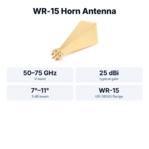
WR-15 Standard Gain Horn Antenna, 50–75 GHz, 25 dBi
$1,299.00 Buy Now
FAQ
What is the difference between range resolution and range accuracy?
Resolution is how close two targets can be and still be separated, c/2B. Accuracy is how close one target’s reported range is to the truth. With good SNR, accuracy can be a hundred times finer than resolution.
Does zero padding improve accuracy?
It reduces the interpolation bias, so it can improve accuracy at high SNR. It does not improve resolution, and it does not add information.
Why does my radar’s distance reading jitter by a few millimetres?
Noise: the scatter follows 1/√SNR. Averaging more chirps or frames, a stronger reflector or a narrower beam all raise SNR and reduce the jitter.
Is the Cramér–Rao bound always reachable?
Only at moderate to high SNR and only with an unbiased estimator. At low SNR, wrong-bin errors dominate; at very high SNR, systematic errors usually take over.
Sources and method
- D. C. Rife and R. R. Boorstyn, “Single-tone parameter estimation from discrete-time observations”, IEEE Transactions on Information Theory, 1974 (Cramér–Rao bound for frequency).
- J. O. Smith, Spectral Audio Signal Processing, W3K Publishing, 2011, section on quadratic interpolation of spectral peaks.
- M. A. Richards, Fundamentals of Radar Signal Processing, 2nd ed., McGraw-Hill, 2014 (straddle loss, interpolation).
- Figures and animations are computed in Python from the formulas shown; the simulation code is open source in Kymopsis/radar-basics-sim. Figures marked SIMULATION are not measurements of a product.