Radar Principles 17: Beamforming and Phased Arrays

Feed eight antennas λ/2 apart with the same signal and they form a beam straight ahead. Delay each one by 90° of phase more than its neighbour and the same beam points 30° to the side, without anything moving. Beamforming is the weighting of many antenna channels so that their signals add up in one direction and cancel in others. A phased array does it with analog phase shifters behind each element; digital beamforming does it with numbers after every channel has been sampled. The physics is the same path-difference argument as angle finding, run in reverse.

This is chapter 17 of Radar Principles, and the most textbook-like one. The angle chapter read a target’s direction from the phase differences across receivers; the MIMO chapter built bigger virtual arrays. Here the question is turned around: given an array, how do you choose the weights so it looks in one direction, ignores another, and keeps its sidelobes down?

Arrays add arrows

Several people pushing a stalled car only move it if they push at the same moment; if half push while the others pause, the effort is wasted. Antennas add their signals the same way: in step they add up, out of step they cancel, and in some directions they cancel completely.

Every antenna in an array delivers the same echo with its own phase, an arrow in the I/Q plane of chapter 2. Beamforming adds the arrows. If they all point the same way the sum is as long as all of them together; if they point in different directions they partly or completely cancel. The way the sum changes with direction is the array factor, and it is the whole of beamforming in one picture.

Straight ahead, every element sees the wave at the same moment, the arrows line up and the sum is 4. At 15° each element is 47° behind its neighbour (chapter 12 gives the rule), the arrows curve and the sum drops to 2.5, about 4 dB down. At 30° the step is 90°, four arrows make a closed square and the sum is zero: the array is deaf in that direction. Further out the arrows wrap around more than once and the sum grows a little again: a sidelobe.

Two consequences follow directly. More elements make the arrows curl shut at a smaller angle, so the beam gets narrower. And if the receiver deliberately rotates each arrow back before adding, the arrows line up for a different direction instead: that is steering, the subject of the next section.

Steering with phase

A stadium wave travels round the stands because each person stands up a moment after their neighbour. Feed each antenna a little later than the one beside it and the combined wave leaves at an angle; change the delay and the beam swings, with nothing moving.

A wave leaving an array at angle θ₀ must have the same phase along a tilted wavefront. Element n, at position n·d, is n·d·sin θ₀ closer to that wavefront than element 0, so it must be fed that much later: a phase lag of 2π·n·d·sin θ₀/λ. For d = λ/2 the step between neighbours is 180°·sin θ₀. On receive the same weights, applied before summing, line up the phases of an echo from θ₀ so they add coherently, while echoes from other directions add with mixed phases and partly cancel.

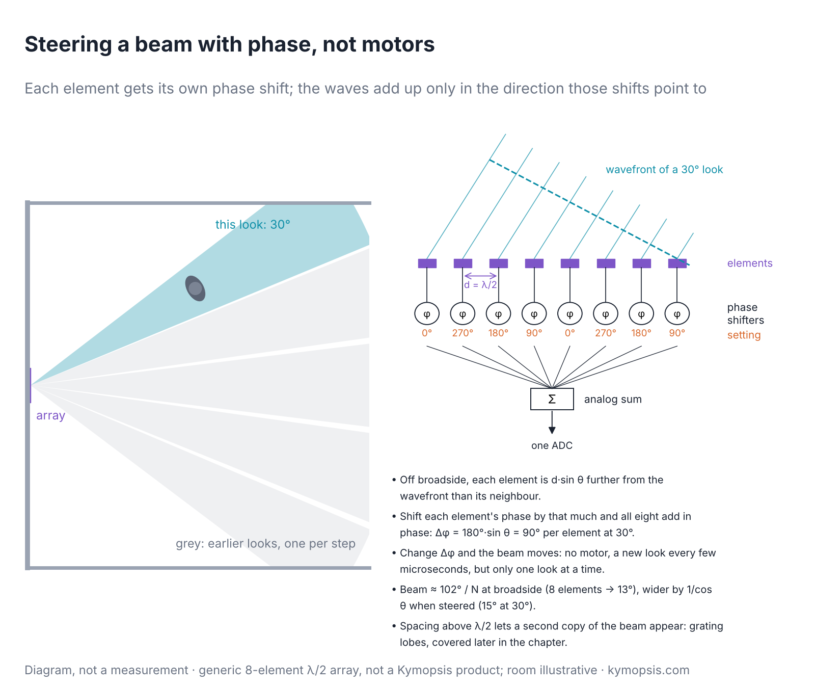
Two numbers describe the main beam. Gain: on receive, N channels add signal coherently and noise incoherently, a factor N in SNR (9 dB for 8, 15 dB for 32). On transmit with one amplifier per element, N amplifiers also add their power and the array concentrates it in the beam, so EIRP grows as N²: 18 dB for 8 elements over a single one. Beamwidth: about 0.886·λ/(N·d) radians at broadside for uniform weights, 12.8° for 8 elements, 6.4° for 16. When the beam is scanned the array looks shorter from the side, and the beamwidth grows as 1/cos θ₀: 18.4° for 8 elements at 45°. The element pattern also falls off away from broadside, so a scanned beam loses gain too.

Grating lobes

Look through a fence with wide gaps and you can see the same lamp through several gaps at once. Antennas spaced too far apart have the same problem: the beam appears in extra directions, as strong as the real one.

The angle chapter showed that spacing wider than λ/2 makes angle readings ambiguous. For a beamformer the same effect is visible: the array factor repeats every time the phase step wraps by 360°, and when a repeat falls inside visible space (between −90° and +90°) the array has a second full-strength beam, a grating lobe.

The rule is d < λ/(1 + |sin θ_max|) for a beam that must scan to ±θ_max: 0.67λ for ±30°, 0.59λ for ±45°, 0.5λ for full ±90°. Arrays that only need a narrow scan, or whose elements are themselves directive enough to suppress the lobe, can space elements more widely and save channels. Sparse arrays and MIMO virtual arrays with gaps rely on this, and on processing that tells the true beam from its copies; the ambiguity chapter covers that side.

Sidelobes and tapering

A choir sounds smoother when the singers at the ends sing a little softer than those in the middle. Tapering an array works the same way: turn down the antennas at the edges and the faint side beams fall away, at the cost of a slightly wider main beam.

Uniform weights give the narrowest beam for a given aperture but a first sidelobe only 13 dB below the peak. In a radar, a strong reflector 13 dB down a sidelobe looks like a weak target in the main beam. Tapering the amplitude, strongest in the centre and weaker towards the ends, lowers the sidelobes at the cost of a wider beam and a little less gain.

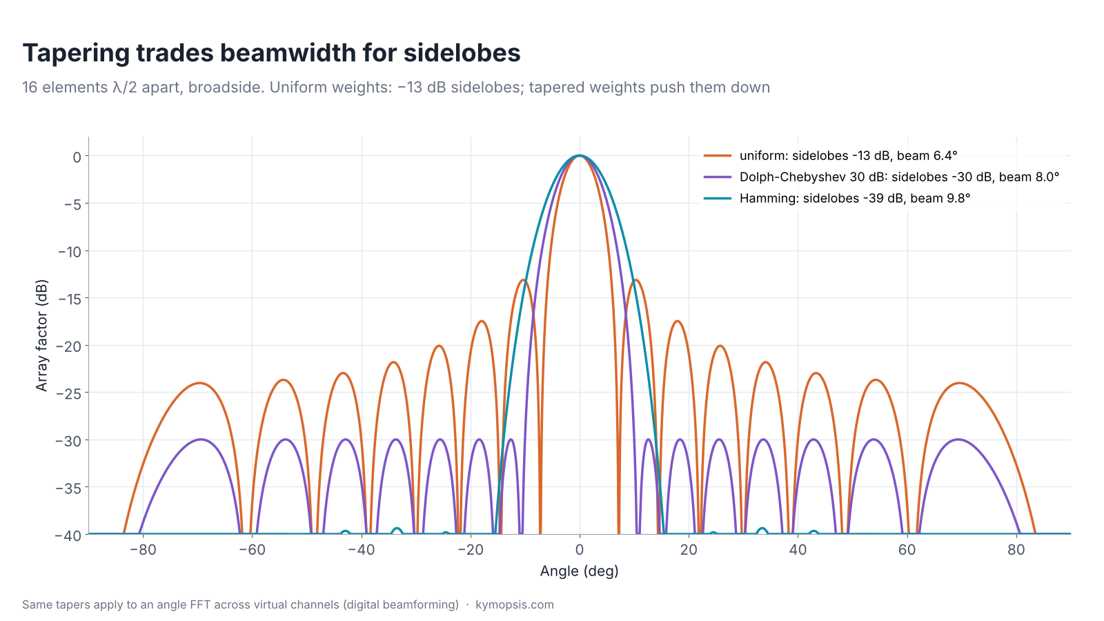
These are the same windows used on the range and Doppler FFTs, and for the same reason. In a digital radar the angle FFT across channels is a beamformer evaluated at every angle at once, so the taper is just a set of numbers multiplied in before the FFT.

Phase shifters, true time delay and beam squint

A phase shifter delays each antenna by a fixed fraction of a wave, not by a fixed time, a bit like a metronome set for one song. It is right at one frequency, and as a chirp sweeps up the band the beam slowly drifts.

A phase shifter delays a signal by a fixed phase, not a fixed time. That is right at one frequency only. An FMCW radar sweeps several gigahertz, so a beam steered with phase shifters points slightly differently at the start and end of each chirp: with fixed phase weights, sin θ(f) = (f₀/f)·sin θ₀.

Across 57–64 GHz the beam moves by 6.7°, about three-quarters of a 16-element beamwidth; for 76–81 GHz at 45° it moves from 46.9° to 43.3°. Small arrays with wide beams barely notice. Large arrays with narrow beams and wide sweeps do, and use true time delay (lines whose delay is the same at every frequency) for at least part of the steering, at the cost of size and loss. Digital beamforming is far less affected on receive: weights applied after the range FFT act at the centre frequency, and small arrays see only slight smearing. Large wideband arrays can apply frequency-dependent steering per fast-time sample before the range FFT.

Phase shifters are also quantised. With n-bit shifters the phase is rounded to 360°/2ⁿ steps, which raises sidelobes: in our 16-element example steered to 17°, 2-bit shifters leave a −8 dB lobe, 3-bit −12.6 dB, 4-bit already close to the ideal −13 dB. Pointing accuracy is far less affected than sidelobes.

Analog, digital and hybrid

A mixing desk can blend all the microphones into one output, or record every microphone on its own track and mix it later in any way you like. Analog arrays do the first and point one beam at a time; digital arrays record every channel and form every beam afterwards.

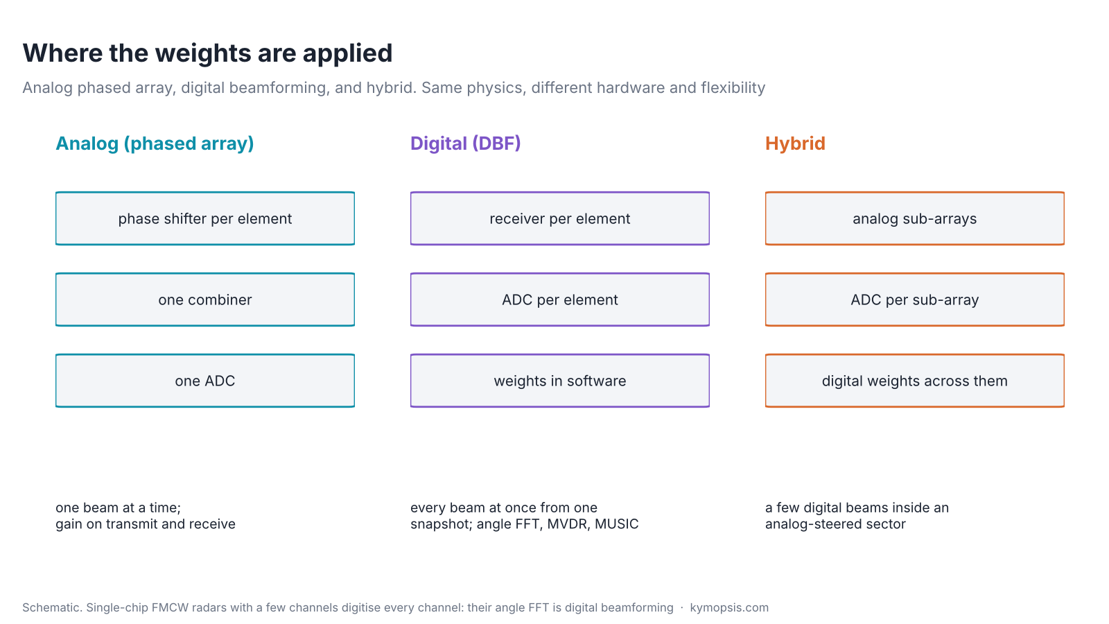
An analog phased array combines the elements in RF hardware and digitises one signal. It forms one beam at a time and needs only one receiver and ADC, and on transmit it really concentrates power in the beam. It must scan to look around, which takes time.

Digital beamforming (DBF) digitises every channel and forms beams in software. One snapshot gives every beam at once, and the weights can change for every range-Doppler cell. The angle FFT in a single-chip FMCW radar is exactly this: the 2T2R modules we sell, like most small radar SoCs, digitise each receive channel and do all their angle processing digitally. The cost is one receive chain and ADC per channel and the data rate that comes with it.

Hybrid arrays steer analog sub-arrays and digitise each sub-array, getting a few digital beams inside an analog-steered sector. Large communication and radar arrays use this to keep the number of ADCs manageable.

Adaptive beamforming: steering nulls

Noise-cancelling headphones listen to the hum around you and play it back against itself. An adaptive array does the same with direction: it measures where the interference comes from and turns a deaf spot towards it, while keeping its ear on the target.

Fixed weights treat every direction the same. Adaptive beamforming (ABF) computes the weights from the data, so the array also points nulls at whatever interferes. The standard form is the minimum-variance distortionless response (MVDR, also called the Capon beamformer): keep unit gain towards the look direction and minimise everything else in the output.

w = R⁻¹·a(θ₀) / (aᴴ(θ₀)·R⁻¹·a(θ₀))

R is the covariance matrix of the channel signals, estimated from many snapshots, and a(θ₀) is the steering vector of the look direction. Where R contains a strong interferer, R⁻¹ is small along it, and the weights put a deep null there.

The price is in the data: R must be estimated from enough snapshots, ideally without the wanted target (with it present, small steering errors make MVDR suppress the target), and with few snapshots or errors in the steering vector MVDR is fragile. Diagonal loading, adding a small constant to R before inverting, is the usual safeguard. Scanned over all angles, the MVDR output becomes a high-resolution spectrum, the Capon method of the super-resolution chapter.

Try it yourself: examples/ch17_beamforming.py in the open-source radar-basics-sim repository runs the core simulation of this chapter; change the assumptions and see what moves.

Where this shows up in what we sell

A torch with an adjustable head narrows its beam by shape alone, with no electronics. The horn and lens on our level kit do the same, giving a fixed narrow beam from size alone, while the 60 GHz boards keep a wide view.

We do not sell phased-array radars or beam-steering modules. The principles still explain hardware we do sell. Our 60 GHz radar modules have two receive channels; their wide-beam elements give the ±60° field of view stated in the datasheet. The 60 m board of our 80 GHz level radar kit takes the opposite route: a horn and PTFE lens give a fixed, narrow beam by aperture alone, the way a dish does, with no steering at all. The trade-offs of aperture, gain and sidelobes are the same, and the antenna chapter works through them for that kit.

GitHub · Kymopsis /radar-basics-simView repository → B2B engineering · KymopsisNeed a narrower beam or a custom antenna?Describe your range, field of view and housing. We scope antennas, lenses and radar modules for B2B projects.Describe your requirement

FAQ

What is the difference between beamforming and a phased array?

Beamforming is the general idea of weighting and combining antenna channels. A phased array is one way to do it, with phase shifters in the RF path. Digital beamforming does the same weighting after sampling every channel.

What causes grating lobes?

Element spacing too large for the scan angle: the phase step between elements wraps by 360° inside visible space and the beam appears again. Keeping d below λ/(1 + |sin θmax|) avoids them.

Is MIMO radar the same as beamforming?

No. MIMO creates a larger virtual array by separating transmitters; the angle processing on that array is digital beamforming on receive. A MIMO radar with orthogonal transmissions does not focus transmit power, while a phased array does.

What is MVDR beamforming?

Minimum-variance distortionless response: adaptive weights that keep unit gain in the look direction and minimise output power from everywhere else, which places nulls on interferers. It is also called the Capon beamformer.

Why does a phased array beam move with frequency?

Phase shifters apply a fixed phase, which equals the needed time delay at one frequency only. At other frequencies of the sweep the beam points elsewhere: beam squint. True time delay avoids it.

Sources and method

• R. J. Mailloux, Phased Array Antenna Handbook, 3rd ed., Artech House, 2017.
• H. L. Van Trees, Optimum Array Processing, Wiley, 2002: array factor, tapers, MVDR.
• P. Delos, B. Broughton, J. Kraft, “Phased Array Antenna Patterns—Part 1”, Analog Devices Analog Dialogue 54-02, 2020 (analog.com): beam squint, grating lobes and quantisation explained with patterns.
• J. Capon, ‘High-resolution frequency-wavenumber spectrum analysis’, Proc. IEEE, 1969.

All figures are computed from the array factor of isotropic elements or simulated with the Kymopsis Radar Principles scripts (ch17_beamforming.py). The chapter stays at textbook level and describes no specific phased-array product.