Radar Principles 18: Super-Resolution with Capon, MUSIC and ESPRIT

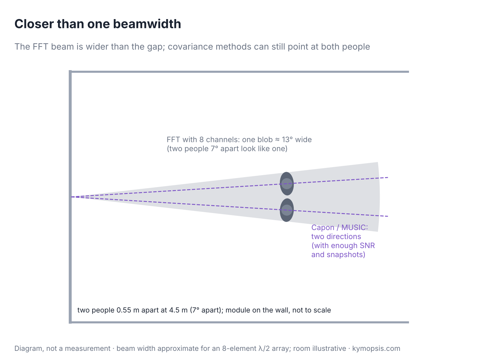
Eight receive channels half a wavelength apart resolve two targets only when they are about 14° apart (by the 3 dB-dip test, about 17°). Put them 6° apart and the angle FFT shows a single lobe. Feed the same data to MUSIC and two sharp peaks appear at the right angles. Super-resolution methods beat the FFT’s 2/N limit by assuming a model, a known number of point targets in white noise, and fitting it to the covariance of many snapshots. When the assumptions hold they work remarkably well; when SNR, snapshots or calibration fall short they fail more abruptly than the FFT.

This is chapter 18 of Radar Principles. The angle chapter gave the FFT limit of about 2/N radians, MIMO raised N, and the beamforming chapter introduced the adaptive Capon (MVDR) beamformer. This chapter asks what can be had beyond the aperture, and what it costs.

Why the FFT stops at 2/N

Two car headlights far down a road blur into one light, and no amount of squinting splits them, because the eye’s lens is only so big. An FFT across a radar’s antennas has the same fixed blur, set by how wide the array is, and a brighter scene does not sharpen it.

The FFT across channels is a fixed linear filter bank: each output is the array steered to one angle with uniform weights. Its beam has a finite width, about 0.886·λ/(N·d), and two targets inside one beamwidth produce a single merged lobe. More SNR does not help, because the shape of that lobe is set by the aperture, not by the noise. To go further, the processing must use something the FFT ignores: how many targets there are, and the fact that each is a pure plane wave.

What a covariance matrix is

Watch a row of dancers for a while and note which pairs move together, and with what delay. That table of who moves with whom is a covariance matrix: one dancer leading gives one neat pattern, two leaders lay two patterns on top of each other.

Capon and MUSIC do not work on the snapshots directly. They first boil the snapshots down to a table, the covariance matrix R. For N channels it has N rows and N columns. Entry (i, k) is the average, over many snapshots, of channel i’s value times the complex conjugate of channel k’s: how strongly the two channels move together, and with what phase offset between them.

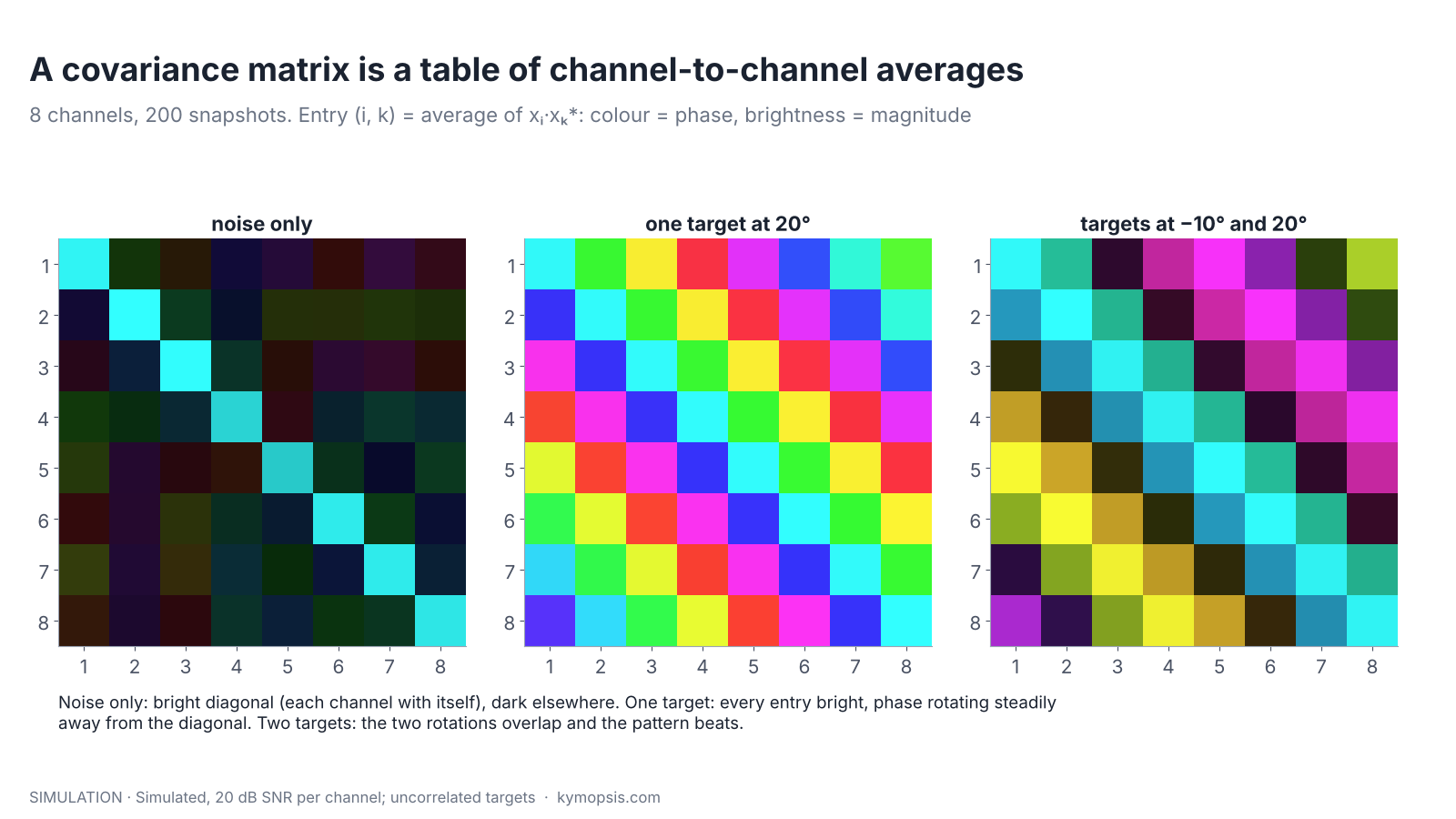
The three cases in the figure show what the table holds. With noise only, each channel agrees with itself (the bright diagonal) and with nobody else, because independent noise averages away. With one target, every channel pair is correlated, and the phase offset between channels i and k is the same angle-dependent step that chapter 12 measured, repeated k − i times. Two targets superimpose two such patterns. R therefore contains the angles of everything in the scene, already averaged over many snapshots; the methods below are different ways of reading them out of it. That averaging is also why they need many snapshots and why echoes that are copies of each other (coherent) confuse them.

Capon: adaptive beamforming at every angle

A sound engineer aiming a directional microphone at a singer also turns its deaf side towards the loudest neighbour. Capon does that at every angle in turn, so a strong target close by does not spill into the view.

Capon’s method scans the MVDR beamformer over all angles and plots its output power, P(θ) = 1/(aᴴ(θ)R⁻¹a(θ)). Because the weights are recomputed for each look direction to null everything else, a nearby target that would leak into an FFT beam is suppressed, and the peaks get narrower. It needs the covariance matrix R, which means many snapshots, and it still has a resolution limit that shrinks with SNR rather than vanishing.

MUSIC: look for what is orthogonal to the noise

To find two singers in a dark hall, you can also listen for where they are not: every direction without a singer sounds like plain background. MUSIC maps the background and points at the gaps in it.

MUSIC (multiple signal classification) splits the covariance matrix into two subspaces. With K targets and N channels, the eigenvectors of the K largest eigenvalues span the directions the echoes come from (the signal subspace), and the remaining N − K span the noise subspace. A steering vector a(θ) that points at a real target lies entirely in the signal subspace and is therefore orthogonal to every noise eigenvector. MUSIC plots

P(θ) = 1 / ‖E_nᴴ · a(θ)‖²

which shoots up wherever that orthogonality holds. The peaks are not power: their height says how well the model fits, not how strong the target is. Amplitudes have to be estimated separately once the angles are known.

ESPRIT: no search at all

ESPRIT uses the same signal subspace but exploits the array’s shift structure: the first N − 1 elements and the last N − 1 elements see the same signals with a phase rotation that depends only on the angles. Solving for that rotation gives the angles directly, without scanning a grid, which makes it cheap and very accurate on uniform linear arrays. Root-MUSIC gets a similar benefit by solving a polynomial instead of searching.

Sparse methods

A newer family treats angle estimation as finding a few non-zero entries in a fine grid of possible angles (compressed sensing, iterative adaptive approaches). These work with fewer snapshots, even one, and handle coherent echoes better, at the price of more computation and parameters to tune. They are used in some imaging radars.

What super-resolution needs

Picking out two quiet voices in a crowd works only if they are loud enough, you listen long enough, and you know how many people are talking. Super-resolution needs the same: enough signal, enough snapshots, the number of targets, and a well-calibrated array.

SNR and snapshots

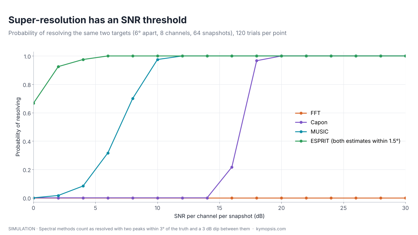
Each method has a threshold: above it, resolution is almost certain; a few decibels below, almost never. In our example with 64 snapshots MUSIC crosses at about 8–10 dB and Capon at about 17–18 dB per channel. ESPRIT’s estimates sit within 1.5° of both targets from very low SNR, though that is a different test from seeing two peaks. Fewer snapshots raise all the thresholds, because the covariance estimate gets noisier. In a radar, snapshots come from successive chirps, frames or neighbouring range cells, and each source has trade-offs: frames take time, during which targets move.

Incoherent echoes, or spatial smoothing

MUSIC assumes the targets’ echoes vary independently from snapshot to snapshot. Radar echoes often do not. Two reflectors in the same range-Doppler cell, or a target and its multipath, keep a fixed phase relation in every chirp: they are coherent. The covariance matrix then has rank one for both of them together, the signal subspace collapses, and MUSIC returns one peak in the wrong place.

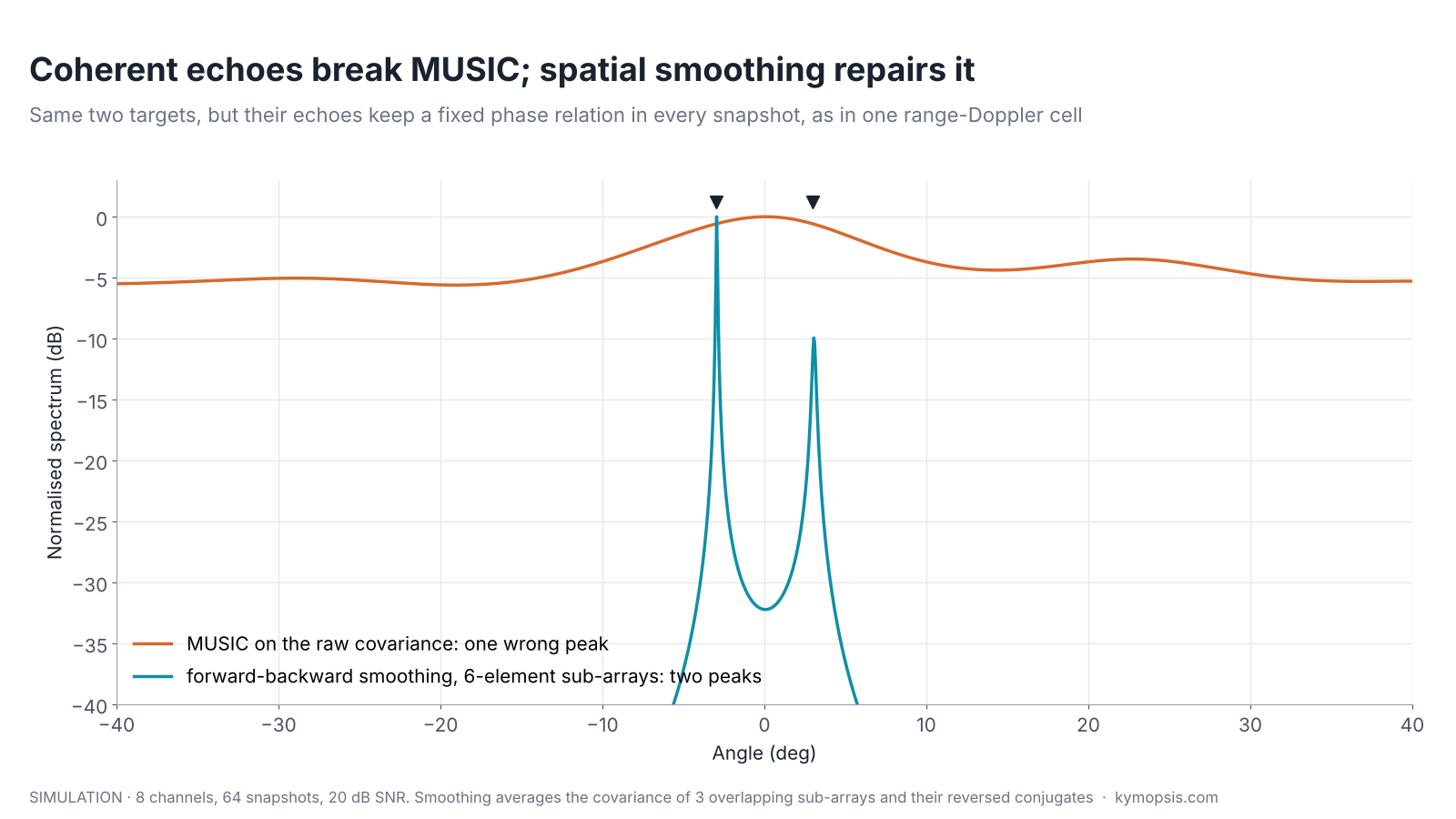
Spatial smoothing restores the rank by averaging the covariance of several overlapping sub-arrays (and, in the forward-backward variant, their reversed conjugates). The relative phase of the two echoes differs from one sub-array to the next, which decorrelates them. It costs aperture: smoothing an 8-element array with 6-element sub-arrays leaves the resolution of six elements. With enough SNR it even works on a single snapshot, which makes single-frame super-resolution possible at high SNR.

The right number of targets

MUSIC and ESPRIT need K, the number of targets, up front. Assume too few and the targets merge or vanish; too many and spurious peaks appear in noise. K is usually estimated from the eigenvalues, with information criteria such as MDL or AIC: in our example MDL correctly finds two incoherent targets, and finds one when the echoes are coherent, which is exactly the failure above.

Calibration

Super-resolution leans on the exact shape of the steering vector. A small phase error per channel, harmless for an FFT, distorts the subspaces. In our simulation at 25 dB SNR, 2° RMS of random channel phase error still allows MUSIC to resolve every time; 5° drops it to about one trial in four; 10° to none. Mutual coupling, a radome that is not uniform over the array, and near-field targets have the same effect, which is why super-resolution is used carefully in production and almost always after calibration.

How the simulation counts ‘resolved’

For FFT, Capon and MUSIC: the two highest peaks of the spectrum each lie within 3° (half the separation) of a true angle, and the spectrum dips by at least 3 dB between them. For ESPRIT, which returns numbers rather than a spectrum: both estimates within 1.5° of the true angles. Snapshots have independent random target phases unless stated as coherent; noise is complex white Gaussian with the stated SNR per channel and snapshot. The script ch18_super_resolution.py prints every figure in this chapter.

Beyond angle

Two piano notes close together blur in a short recording, but if you know each is a pure note you can still tell there are two. The same reasoning separates two targets closer than one range bin.

Nothing above is specific to angle. A range profile is also a sum of complex exponentials, one per target, sampled across the ADC samples of a chirp, so MUSIC, ESPRIT and sparse methods can split targets closer than c/2B in range and closer than the Doppler resolution in velocity. The same conditions apply: SNR, a known model order, and a well-behaved signal. In practice, range super-resolution is limited by the sweep’s linearity and by targets that are not points. The sub-bin range precision chapter covers the simpler and more robust job of locating one target inside a bin.

Try it yourself: examples/ch18_music_vs_fft.py in the open-source radar-basics-sim repository runs the core simulation of this chapter; change the assumptions and see what moves.

On small radars

A magnifying glass cannot show more than its lens gathers. With only a few channels a small radar has little to work with, and super-resolution pays off on large arrays looking at few targets.

With the four virtual channels of a 2T2R module such as our 60 GHz AiP radar or PCB-antenna radar, MUSIC can in principle separate at most three targets in one cell and needs high SNR and good calibration to beat the FFT by much. The module firmware does its own angle processing and the datasheets do not say which method it uses, so we make no claim about it. Super-resolution matters most when the array is already reasonably large and the scene is sparse, which is why it is common in automotive and 4D imaging radars.

GitHub · Kymopsis /radar-basics-simView repository → B2B engineering · KymopsisNeed to separate close targets?Describe the targets, distances and array size you can afford. We scope radar hardware and processing for B2B projects.Describe your scene

FAQ

Can MUSIC beat the Rayleigh resolution limit?

Yes, given enough SNR and snapshots, uncorrelated (or decorrelated) echoes, a correct target count and a calibrated array. Below its SNR threshold it fails more abruptly than the FFT.

What is the difference between MUSIC and Capon?

Capon scans an adaptive beamformer and its output is power; MUSIC tests orthogonality to the noise subspace and its peaks are not power. MUSIC usually resolves at lower SNR but needs the number of targets; Capon does not.

Why does MUSIC fail on radar data from one range-Doppler cell?

Echoes in one cell are coherent, so the covariance matrix loses rank. Spatial smoothing over sub-arrays restores it at the cost of aperture.

Does super-resolution work with a single chirp?

Covariance-based methods need several snapshots, or spatial smoothing to create them from one. Sparse (compressed-sensing) methods are designed for single-snapshot use.

Sources and method

• R. O. Schmidt, ‘Multiple emitter location and signal parameter estimation’, IEEE Trans. Antennas Propag., 1986.
• R. Roy, T. Kailath, ‘ESPRIT: estimation of signal parameters via rotational invariance techniques’, IEEE Trans. ASSP, 1989.
• T.-J. Shan, M. Wax, T. Kailath, ‘On spatial smoothing for direction-of-arrival estimation of coherent signals’, IEEE Trans. ASSP, 1985.
• M. Wax, T. Kailath, ‘Detection of signals by information theoretic criteria’, IEEE Trans. ASSP, 1985.
• H. L. Van Trees, Optimum Array Processing, Wiley, 2002.

All figures are simulated with the Kymopsis Radar Principles scripts (ch18_super_resolution.py, using the shared capon() and music() functions): an 8-element λ/2 array, narrowband snapshots, complex white noise. None is measured data.