


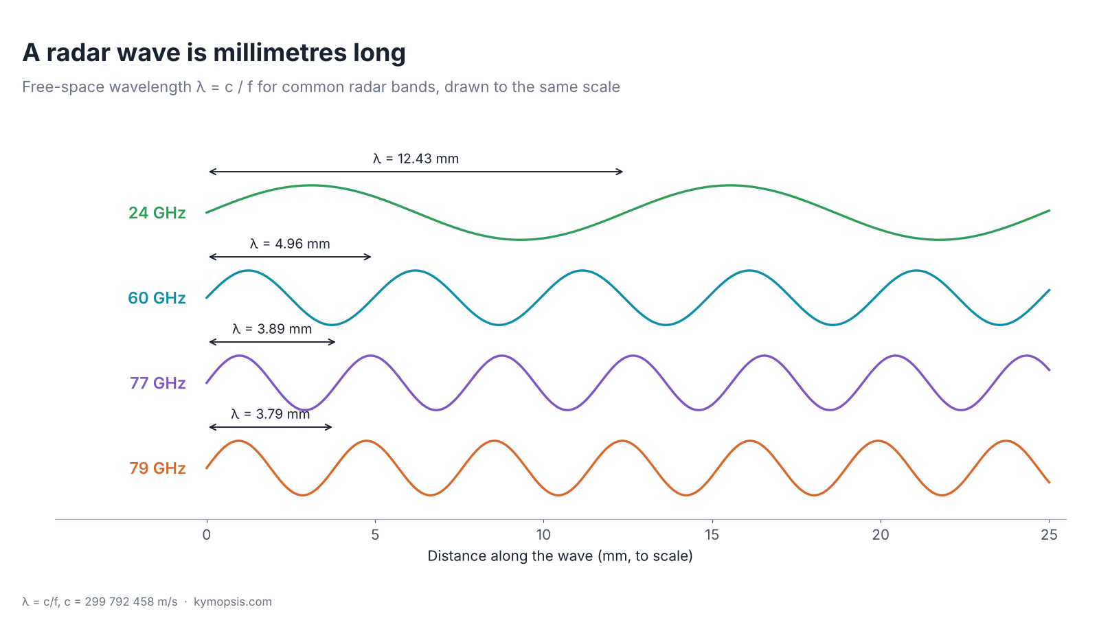
A 60 GHz radar module sends out a wave whose crests are 4.96 mm apart. Everything that comes later in this series, the range resolution, the micrometre phase readings, the size of the antenna, how much a plastic cover gets in the way, follows from that one length and from how the wave is launched. This first chapter covers where the wave comes from, how it spreads, and why the echo that comes back is so small.
What a radar does, in one paragraph. It sends out a radio wave; part of the wave bounces off a target, a person, a hand or a liquid surface, and comes back. Because the echo travels out and back, it returns after a delay τ = 2R/c, where R is the distance and c the speed of light. A person 3 m away answers after 20 ns; moving them 1 mm further delays the echo by only 6.7 ps. Reading that delay, and how it changes from one moment to the next, is what every later chapter is about.
What a radio wave is
Drop a pebble in a pond: rings run outward, yet the water itself only bobs up and down where it is. A radio wave is the same kind of travelling pattern, made of electric and magnetic field instead of water, so it needs no water, no air, nothing at all to travel through. The gap between two rings is what engineers call the wavelength, and the number of rings passing a point each second is the frequency.
Same wave, different length. Your phone, your Wi-Fi router, a microwave oven and the radar in a car all send out this same kind of wave; only the frequency differs. Phones work around 0.9 GHz, Wi-Fi and microwave ovens around 2.4 GHz, car radars at 77 GHz. An FM radio wave is about three metres long, Wi-Fi about twelve centimetres, a 60 GHz radar five millimetres, and green light half a thousandth of a millimetre, yet all of them travel at the speed of light.
A radio wave is an electric field and a magnetic field that keep regenerating each other while they travel. The electric field points across the direction of travel, the magnetic field is at right angles to both, and the pattern moves at the speed of light, c = 299 792 458 m/s in vacuum and almost the same in air.
Two numbers describe it. The frequency f is how many times per second the field at one point reverses. The wavelength λ is the distance between two crests at one instant. They are tied together by λ = c/f. At 60.5 GHz that gives 4.96 mm; at 77 GHz, 3.89 mm. That is why radars in the 57–64 GHz and 76–81 GHz bands are called millimetre-wave radars.
| Band | Centre used here | Wavelength λ | Half wavelength λ/2 |
|---|---|---|---|
| 24 GHz ISM | 24.125 GHz | 12.43 mm | 6.21 mm |
| 57–64 GHz | 60.5 GHz | 4.96 mm | 2.48 mm |
| 76–77 GHz | 77 GHz | 3.89 mm | 1.95 mm |
| 77–81 GHz | 79 GHz | 3.79 mm | 1.90 mm |
Keep the last column in mind. Half a wavelength comes back again and again: it is the spacing of receive antennas for angle measurement, the distance a target moves for the echo phase to turn once around, and the step in radome thickness that makes a cover nearly invisible.
How an antenna launches it
Move your hand up and down in a bath and rings spread out from it. An antenna does this with electrons: the transmitter pushes them up and down a piece of metal billions of times a second, and every push sends a ripple of electric and magnetic field outward.
Any electric charge that accelerates radiates. In an antenna the transmitter drives an alternating current up and down a conductor billions of times per second. The changing current makes a changing magnetic field, that makes a changing electric field, and the disturbance peels away from the conductor and travels outward.
Two things are visible in the animation. The field is strongest broadside to the wire and vanishes along its axis: an antenna never radiates equally in all directions. And the rings are one wavelength apart and fade as 1/r, because the same energy is spread over a larger and larger sphere.
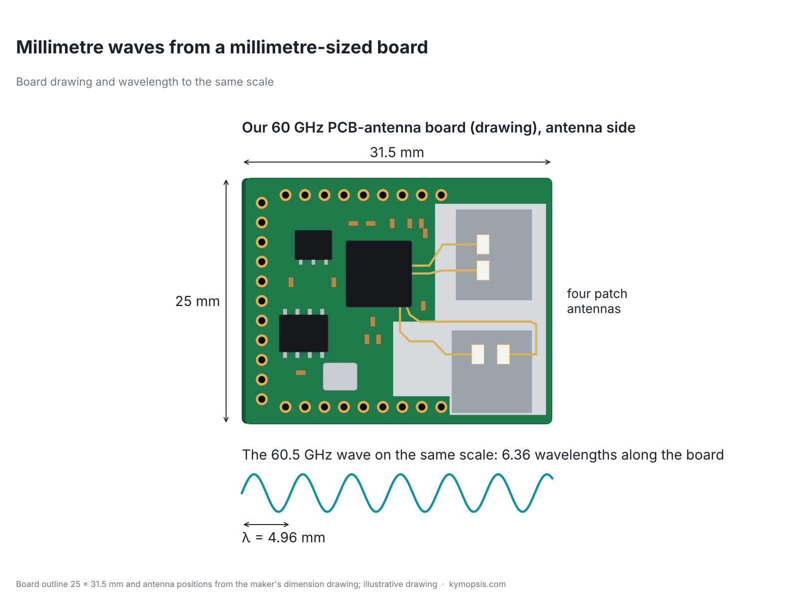
A radar module does not use a bare wire. It uses patch antennas: small copper rectangles on a circuit board above a ground plane. A patch radiates mostly straight out of the board (broadside), which is what a module needs. Several patches side by side form an array that narrows the beam; chapter 4 goes into the different antenna types and chapter 17 into steering a beam with an array.
Think of a bare light bulb and the same bulb inside a torch. The bulb lights the whole room dimly; the torch makes no extra light but puts it all in one bright spot. Antenna datasheets describe this with one number, the gain. An antenna does not create power; it only decides where the power goes. A patch array sends more of it forward and less to the sides, and the gain says how much denser the power is in the best direction than if the same power were spread evenly over a whole sphere. Squeeze all of it into a 12° cone and the density inside is about 365 times higher, which is 26 dB, written 26 dBi (decibels are explained below). How the size of an antenna sets its gain and beamwidth is in chapter 4.
Polarisation
Pass a rope through a fence of upright slats. Shake it up and down and the wave runs through; shake it sideways and the slats stop it. A radio wave also shakes in one direction, and a receiving antenna behaves like that fence: it picks up the wave well only if it is lined up the same way.
The electric field of a wave points in one particular direction across the path, and that direction is its polarisation. A single patch fed on one edge gives linear polarisation: the field swings back and forth in one plane. Feeding a patch at two orthogonal points, driven 90° out of phase, gives circular polarisation, where the field vector rotates as the wave travels.
For a radar this matters in two practical ways. A transmit and a receive antenna must share the same polarisation, or a large part of the signal is lost. And smooth flat surfaces keep linear polarisation on reflection, while edges, wires and rough surfaces can rotate it. When you mount a module, rotating it by 90° around its axis changes which targets look bright.
Near field and far field
Hold your eye close to a torch with several LEDs and you see separate bright spots; walk a few steps back and they merge into one clean beam. Every antenna has the same two zones: close to it the beam has not formed yet, further out it has a fixed shape that no longer changes with distance.
Close to an antenna the field is complicated: part of the energy just sloshes back and forth, and the beam has not formed yet. Far enough away, the wavefronts are nearly flat and the radiation pattern no longer changes with distance. A common rule puts the start of this far field at the Fraunhofer distance
Rff = 2D² / λ, where D is the largest dimension of the antenna.

For a 10 mm patch array at 60 GHz this is about 4 cm, so for room-scale sensing the target is always in the far field. For a 75 mm lens antenna at 79 GHz it is close to 3 m. That is why the near-range readings of large-aperture level gauges behave differently, and why datasheets often state a minimum range.
Where 2D²/λ comes from
The rule says the path difference between the centre and the edge of the aperture, seen from the target, is at most λ/16, i.e. a phase error of π/8 (22.5°). From geometry, a point at range R sees the edge at distance √(R² + (D/2)²) ≈ R + D²/(8R). Setting D²/(8R) = λ/16 gives R = 2D²/λ. A stricter phase error budget pushes the boundary further out.
Decibels: the radar engineer’s units
Decibels are a way of counting zeros. A watt and a picowatt are twelve factors of ten apart; instead of writing 0.000 000 000 001, an engineer counts the factors of ten and multiplies by ten: 120 dB. Each step of ten in power is 10 dB, so huge ratios become two- or three-digit numbers that you can add and subtract in your head.
Before following the wave out to a target and back, it is worth learning the unit that every radar datasheet and every later chapter uses. Radar power levels cover an enormous range: a module might transmit 10 milliwatts and receive an echo of less than a picowatt from a target 10 m away, a ratio of tens of billions. Writing such numbers as plain ratios is clumsy, so engineers use the decibel, a logarithmic scale:
ratio in dB = 10 · log10(P2 / P1)
Three facts make it easy to use in your head. A factor of 2 in power is 3 dB, a factor of 10 is 10 dB, and a factor of 100 is 20 dB. Halving is −3 dB. And because logarithms turn multiplication into addition, a chain of gains and losses is simply added up: 10 dB of gain, then 3 dB of loss, is 7 dB in total.
- dB is a pure ratio: the gain of an amplifier, the loss of a radome, the SNR.
- dBm is an absolute power, referred to 1 milliwatt: 0 dBm is 1 mW, 10 dBm is 10 mW, 30 dBm is 1 W, −30 dBm is 1 µW. Adding a gain in dB to a power in dBm gives a power in dBm.
- dBi (the torch number from above, in decibels) is antenna gain relative to an ideal antenna that radiates equally in all directions (an isotropic radiator). An 8 dBi antenna puts about 6.3 times more power density in its best direction.
- Voltages use 20·log10, because power goes with the square of voltage: doubling an amplitude is +6 dB, and both formulas give the same number of decibels for the same change.

The figure shows why the scale matters. From the transmitter to the echo of a target at 10 m the power drops by about 103 dB, a factor of twenty billion, and the echo is still about 25 dB above the receiver noise in one range bin. In decibels these are small, readable numbers. Chapter 7 builds the full radar equation in exactly this form.
Why the echo is so weak
Shine a torch at a wall, then step back to twice the distance: the spot covers four times the area, so each part of it is four times dimmer. A radar echo pays this price twice, once on the way to the target and once on the way back, so twice the distance means sixteen times less echo.
Now the decibels earn their keep. Power leaving an antenna spreads over a sphere, so the power density falls as 1/R². A target intercepts a small part of it and scatters it in all directions, and the wave coming back spreads again as 1/R². The received power therefore falls as 1/R⁴: double the range and the echo is 12 dB weaker; ten times the range and it is 40 dB weaker. Chapter 7 turns this into the full radar equation and the signal-to-noise ratio that sets every precision limit later in the series.
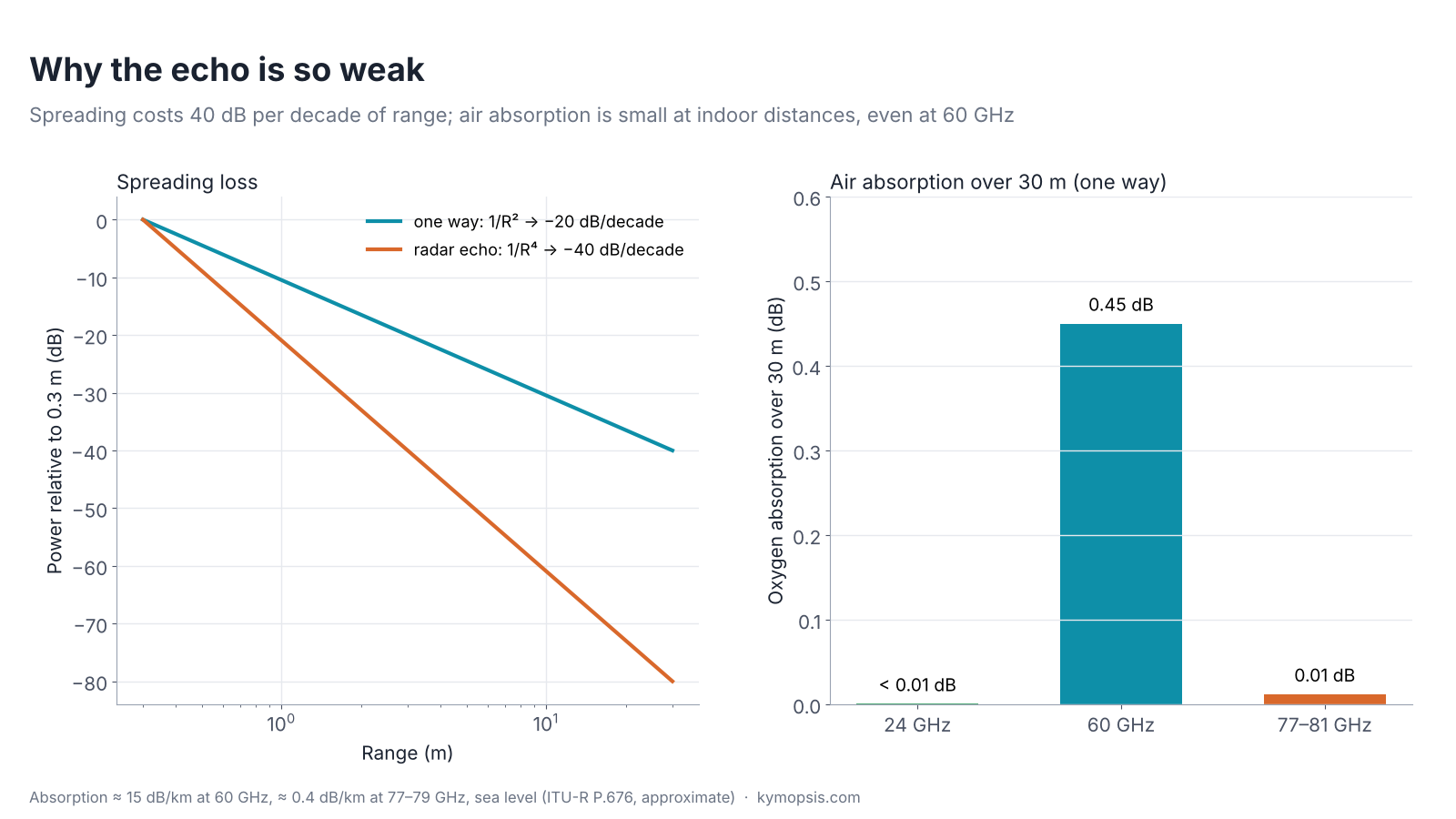
People often hear that 60 GHz is “absorbed by oxygen”. It is, at about 15 dB per kilometre at sea level, which matters for long outdoor links. Over 30 m it is under half a decibel, so indoors it is negligible next to spreading. At 77–81 GHz it is around 0.4 dB per kilometre.
Why millimetre waves make small antennas
A guitar string rings at the note whose half wave fits exactly along it; a shorter string gives a higher note. A patch antenna is the same idea in copper: it works best at the frequency whose half wave fits along the patch, so the higher the frequency, the smaller the antenna.
A patch antenna resonates when its length is about half a wavelength inside the circuit-board material. The material slows the wave by √εr, so the length is roughly λ0/(2√εr).

On a substrate with εr = 3, a patch is about 3.6 mm long at 24 GHz and about 1.4 mm at 60 GHz. That is small enough to put several transmit and receive antennas inside the chip package itself, which is what antenna-in-package (AiP) modules do. The same shrinking is why a complete 60 GHz radar with several antennas fits on a board a few centimetres across, and why the machining tolerances of millimetre-wave parts are so tight (see wavelength, machining tolerance and test cost).
What the receiver does with the echo. The echo that comes back is the same wave, only much weaker and a little late. No converter samples a 60 GHz wave directly, so the receiver compares the echo with the signal it is sending at that moment and turns the difference into two slow voltages, called I and Q. How that comparison works, and why a lag of a fraction of one cycle reveals micrometres of motion, is chapter 2.
Try it on real hardware
The 60 GHz boards we sell are a direct way to see these numbers. The pre-flashed AiP gesture sensor carries its antennas inside the chip package; the PCB-antenna development kit uses patch antennas on the board. The 80 GHz level kit puts a lens or horn in front of the radar to narrow the beam, which is the far-field trade-off above in practice.
Try it yourself: examples/ch01_wavelength.py in the open-source radar-basics-sim repository runs the core simulation of this chapter; change the assumptions and see what moves.
-

60 GHz AiP Gesture & Presence Radar Sensor Module, Pre-flashed (57–64 GHz, 2T2R)
From $19.00Sensor onlySensor + USB-TTL adapter (3.3 V LDO)Reset optionsGesture recognitionPresence, ceiling mountPresence, wall mountPresence and fall events, ceiling mountBreathing and heart rate (research)Select options This product has multiple variants. The options may be chosen on the product page -

60 GHz Gesture & Presence Radar Module Development Kit, PCB Antenna (2T2R, 25 × 31.5 mm)
From $19.00DIY boardDevelopment kitReset optionsGesture recognitionPresence, ceiling mountPresence, wall mountPeople countingPresence and fall events, ceiling mountBreathing and heart rate (research)Select options This product has multiple variants. The options may be chosen on the product page -
WR-12 Rectangular Waveguide Standard Gain Horn Antenna 20 dBi Typical Gain, E Band 60 to 90 GHz
$2,079.00 Buy Now
FAQ
Is 60 GHz radar safe?
The modules in this series transmit milliwatt-level power within the limits of their radio rules. Millimetre waves do not ionise and penetrate skin by well under a millimetre. Exposure limits are set by bodies such as ICNIRP and the FCC; check the module’s own documentation for its output power.
Why do radars use 24, 60 and 77–81 GHz specifically?
These are the bands regulators allocate for short-range and vehicle radar. Higher frequency allows wider sweep bandwidth (finer range resolution) and smaller antennas. Chapter 20 compares the bands in detail.
Does a millimetre-wave radar see through walls?
Barely. Plastic, glass and thin wood pass most of the signal, brick and concrete absorb most of it, and metal and water reflect it. Chapter 13 shows how to design a cover that the wave passes through cleanly.
What is the difference between wavelength in air and in the circuit board?
In a material the wave slows by √εr, so its wavelength shrinks by the same factor. Antenna and radome dimensions use the wavelength inside the material.
Sources and method
- C. A. Balanis, Antenna Theory: Analysis and Design, 4th ed., Wiley, 2016 (dipole fields, far-field criterion, patch antennas).
- M. I. Skolnik, Introduction to Radar Systems, 3rd ed., McGraw-Hill, 2001 (radar range dependence).
- ITU-R Recommendation P.676, attenuation by atmospheric gases (approximate sea-level values used).
- Figures and animations are computed in Python from the formulas shown; the simulation code is open source in Kymopsis/radar-basics-sim. Nothing in this chapter is a measurement of a product.