Radar Principles 2: Phase, I/Q and the Complex Radar Signal

Move a target 2.48 mm further from a 60 GHz radar and its echo looks exactly the same as before. Move it 1.24 mm and the echo is turned upside down. The quantity that changes is the phase, and it is the most sensitive thing a radar measures: one degree of phase is about seven micrometres of distance. This chapter starts from what a radar receiver actually puts out, builds the two numbers called I and Q from it, reads phase as the angle between them, and only then works out why phase follows distance so finely. It ends with what goes wrong in real receivers.

What the receiver actually puts out

Phase is simply where in its swing a wave is at a given moment. Picture the wave as a clock hand that goes round once per cycle: at the radar the transmitted wave is at, say, twelve o’clock, and the echo that comes back from the target may arrive at three o’clock. That offset, a quarter turn or 90°, is the echo’s phase. The radar cannot watch the hand directly at 60 billion turns a second, so it compares the echo with the wave it is sending at that moment, and the comparison is the subject of this section.

A radar cannot watch a 60 GHz wave directly: no analogue-to-digital converter samples that fast. Instead it compares the echo with the signal it is transmitting at that moment, in a mixer, a circuit whose output is the product of its two inputs. Multiplying two cosines gives two new tones, one at the difference of their angles and one at the sum:

cos a · cos b = ½ cos(a − b) + ½ cos(a + b)

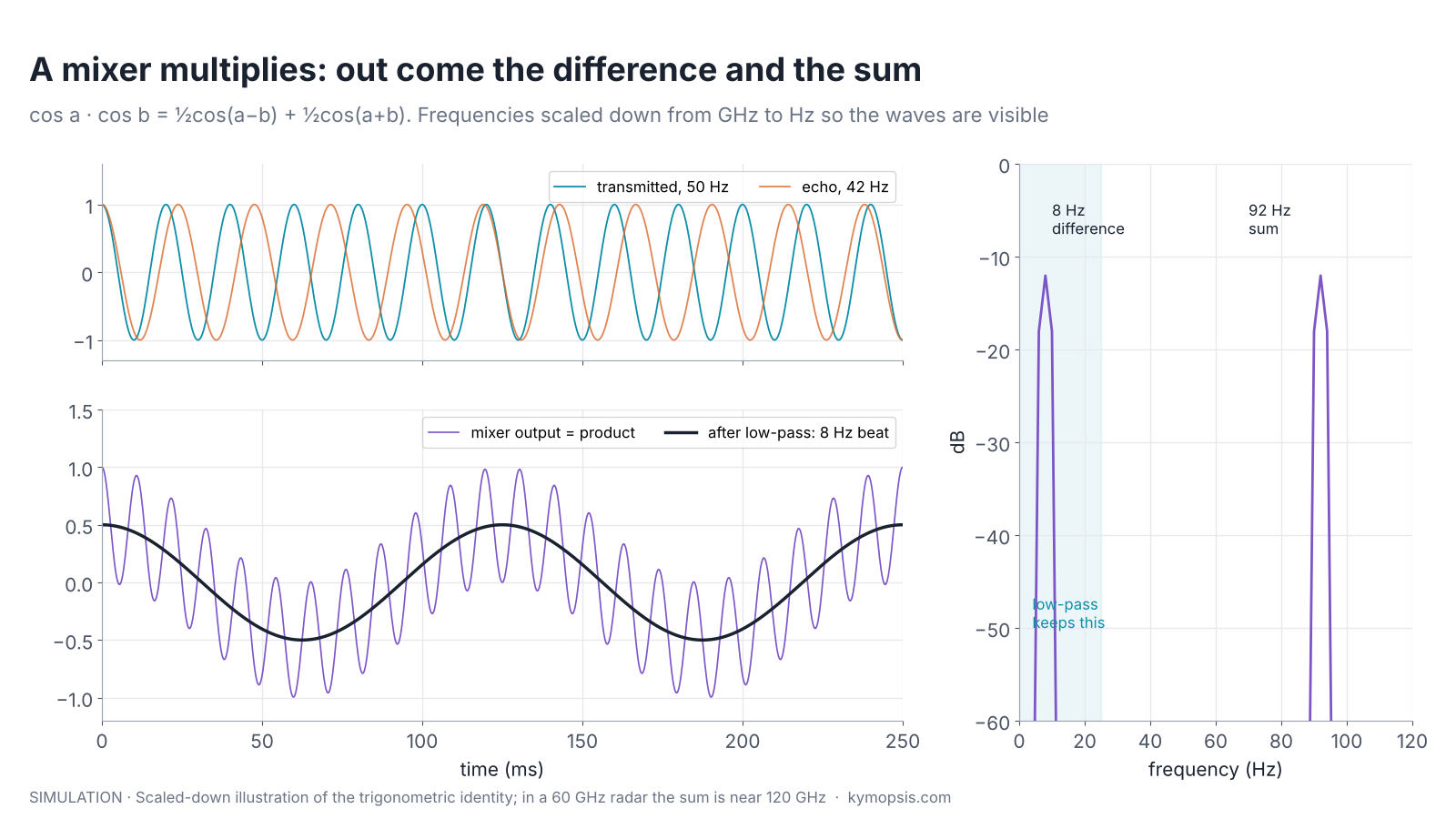
The echo has the same frequency as the transmitter, so the difference term is slow, and a low-pass filter, a circuit that lets only slow signals through, removes the sum term near 121 GHz. What is left is a voltage proportional to cos φ, where φ is how far the echo lags behind the transmitted wave, measured in degrees of one cycle. That lag is the phase of the echo. For a target standing still the output is a constant voltage; move the target and the voltage swings up and down. How a mixer works in a chirping radar is shown step by step in chapter 5.

One such voltage has two blind spots. A reading of half the maximum could mean φ = +60° or φ = −60°, so it cannot tell which way the target moved. And a weak echo at 0° gives the same voltage as an echo twice as strong at 60°, so the strength and the phase of the echo are mixed into one number. A continuous-wave sensor with a single mixer really has these blind spots; an FMCW radar with a single mixer gets around them after the FFT, as the section on real and complex sampling shows.

A second mixer, shifted by 90°: I and Q

Shine a lamp on a turning clock hand and look only at its shadow on the floor: the shadow grows and shrinks, but you cannot tell whether the hand is at two o’clock or four o’clock, because both throw the same shadow. Add a second lamp from the side, so you also see the shadow on the wall, and the two shadows together pin down exactly where the hand points. I and Q are those two shadows.

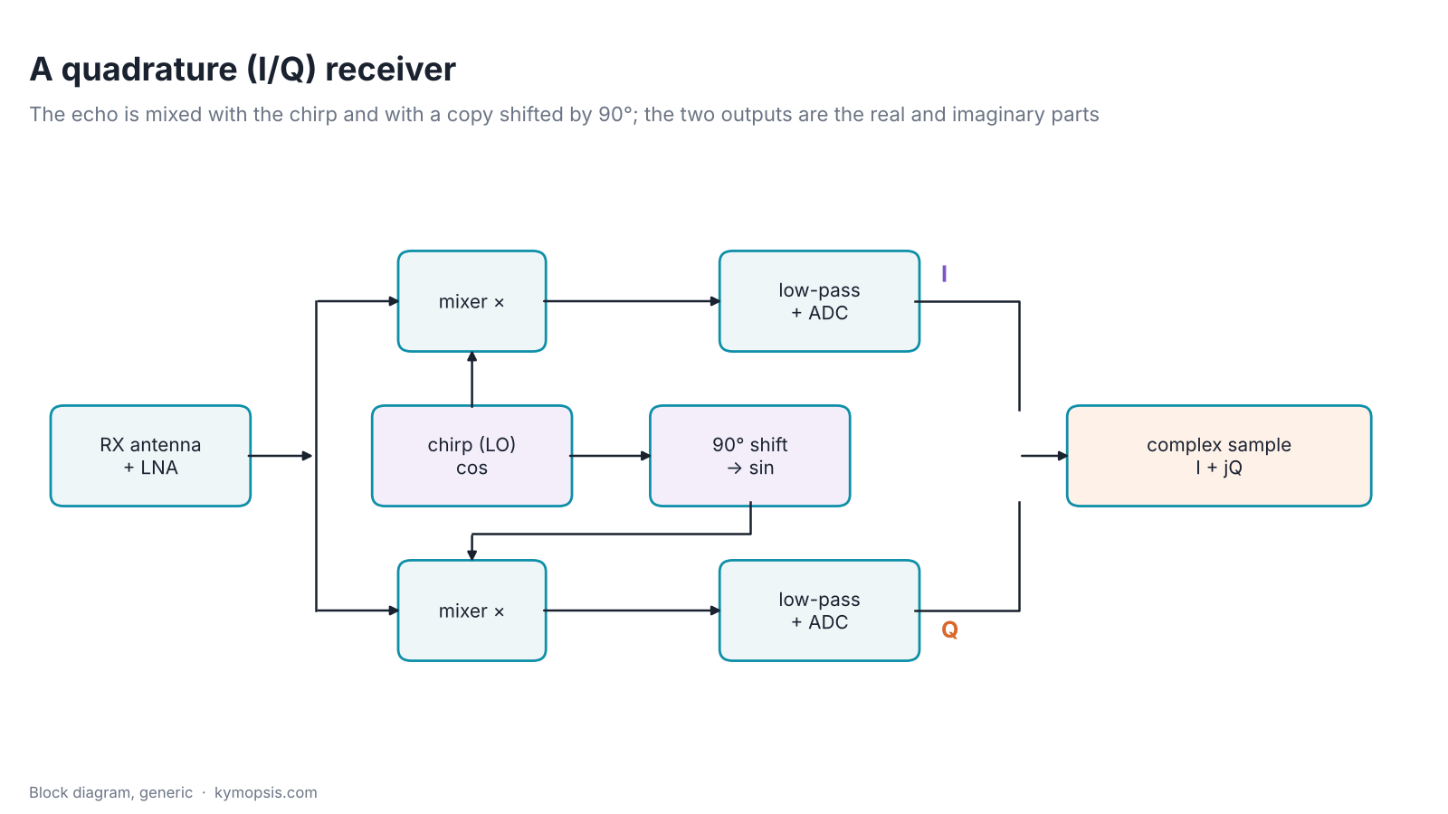
The fix is a second mixer. The received signal is split in two. One half is mixed with the local oscillator (in a radar, a copy of the transmitted signal); the other half is mixed with the same oscillator delayed by a quarter of a cycle, 90°. After low-pass filtering, the first output is I = A·cos φ (in-phase) and the second is Q = A·sin φ (quadrature), up to a sign convention, where A is the strength of the echo. Each output gets its own analogue-to-digital converter.

The 90° shift is the whole trick, and it is also the weak point: it has to be accurate, and the two paths have to have equal gain. How well a chip manages this is part of why some radar chips offer complex (I/Q) sampling and others sample only one real channel per antenna.

Phase is the angle of the I/Q point

Put the two shadows back together and you get the clock hand itself: its length is how strong the echo is, and the angle it points at is the phase.

Plot I on the horizontal axis and Q on the vertical axis, and every pair of readings becomes one point. Its distance from the centre is the echo strength, and its angle from the horizontal axis is the phase:

• amplitude A = √(I² + Q²)
• phase φ = atan2(Q, I), which returns an angle between −180° and +180° and uses the signs of I and Q to pick the right quadrant

This removes both blind spots of the single channel: +60° and −60° now land on different points, and a weak echo sits closer to the centre instead of at a different angle.

Engineers draw this as an arrow from the centre to the point and call it a phasor: its length is the amplitude, its angle the phase, and I and Q are its two shadows. When the target moves, the arrow turns. Every quantity a radar extracts later in this series, range, velocity and angle, ends up being read from either the speed or the angle of such an arrow.

Writing I and Q as one complex number, s = I + jQ = A·e^jφ, is just bookkeeping that makes the algebra short. Multiplying two complex numbers multiplies their lengths and adds their angles, so delays, Doppler shifts and antenna spacings all become simple multiplications. Nothing about the signal is “imaginary”; Q is a voltage measured on a real wire just like I.

Euler’s formula and why the complex form helps

Euler’s formula states e^jφ = cos φ + j sin φ. A tone at frequency f is then s(t) = A e^{j(2πft + φ₀)}. Delaying it by τ multiplies it by e^−j2πfτ, a pure rotation. For the radar echo, τ = 2R/c and f is the carrier, which gives the 4πR/λ phase above. In the real form you would need trigonometric identities for every step; in the complex form you add exponents.

The complex form also makes positive and negative frequencies distinct: e^+j2πft turns anticlockwise and e^−j2πft turns clockwise. A real cosine is the sum of the two, cos(2πft) = ½(e^j2πft + e^−j2πft), which is why its spectrum is mirrored around zero.

Why one channel is not enough

Watch a merry-go-round from the side and you see the horses slide left and right, but you cannot tell which way it is turning. Look from above and the direction is obvious. One channel is the side view; I and Q together are the view from above.

Consider the simplest radar, a continuous-wave (CW) Doppler sensor like the 24 GHz motion detectors in automatic doors. A moving target makes the echo phase turn steadily, so the receiver output is a tone at the Doppler frequency. If the receiver records only I, a target walking towards the sensor and one walking away give the same cosine, because cos(−φ) = cos(φ). The direction of motion is lost.

With I and Q the arrow visibly turns anticlockwise for one direction and clockwise for the other, which is the sign of the Doppler frequency. The same reasoning applies to every measurement that depends on the sign of a frequency or phase change: whether a hand is moving towards or away from a gesture sensor, or whether a chest is rising or falling.

How far the arrow turns when the target moves

Step back by one small step and the echo has two extra steps to travel, one out and one back. Every extra half wavelength of distance, 2.48 mm at 60 GHz, adds a whole wavelength to the round trip and turns the clock hand once all the way round. So the hand turns fast for tiny movements, which is what makes phase so sensitive.

Now put numbers on it. At 60.5 GHz the wavelength is λ = c/f = 4.96 mm. Move the target 1 mm further away. The echo’s path, out and back, grows by 2 mm, which is 2/4.96 = 0.40 of a wavelength. The echo therefore arrives 0.40 of a cycle later, and the I/Q arrow turns by 0.40 × 360° ≈ 145°.

Move the target 2.48 mm instead, and the path grows by 4.96 mm, exactly one wavelength: the arrow makes one full turn and the echo looks exactly as it did before. The same reasoning for a target at any range R, whose echo travels 2R, gives the general formula:

φ = 2π · 2R / λ = 4πR / λ (modulo 2π)

The factor 4π instead of 2π comes from the round trip: the phase completes a full turn when the target moves by λ/2, not λ. At 77 GHz that is 1.95 mm. Divide 2.48 mm by 360 and one degree of phase corresponds to about 6.9 µm at 60.5 GHz.

Band	λ	Motion per phase turn (λ/2)	Motion per degree
24.125 GHz	12.43 mm	6.21 mm	17.3 µm
60.5 GHz	4.96 mm	2.48 mm	6.9 µm
77 GHz	3.89 mm	1.95 mm	5.4 µm
79 GHz	3.79 mm	1.90 mm	5.3 µm

This is the foundation of three later chapters. Phase ranging reads tiny displacements from this angle, Doppler processing reads velocity from how fast the angle turns from one chirp to the next, and angle measurement reads direction from the phase difference between two receive antennas.

Real and complex sampling side by side

Not every radar records both I and Q. Many FMCW radar chips, including some of the modules in this series, have one mixer and one analogue-to-digital converter per receive channel: real sampling. Others have the quadrature pair described above: complex sampling. Both measure range, velocity and angle. Which one a module uses is a chip design choice, not a quality grade, and the datasheet states it.

Why real samples still give I and Q. In an FMCW radar (chapter 5) a target turns into a beat tone whose frequency is set by its range, and the radar takes an FFT of each chirp’s samples (chapter 6). For every frequency bin, the FFT multiplies the samples by two reference tones a quarter cycle apart, a cosine and a sine, and adds up each product. The cosine sum is the I of that bin and the sine sum its Q (up to a sign convention): the same two-mixer trick, done in arithmetic after the ADC. So the value in every range bin is a complex number with an amplitude and a phase even when the ADC recorded a single real channel, and Doppler and angle are read from exactly these values. The direction problem of the single mixer goes away too: velocity comes from how the phase of a range bin turns from one chirp to the next, and that turn has a sign.

The cost is a mirrored spectrum. A real signal contains +f and −f equally, so half of the FFT output is a mirror copy and is discarded, and the receiver cannot tell a positive from a negative beat frequency. For a target in front of an FMCW radar the beat frequency is positive, so nothing is lost in normal use.

	Real sampling	Complex (I/Q) sampling
Hardware per receive channel	One mixer, filter and ADC	Two of each, with an accurate 90° shift and equal gain
Highest beat frequency at ADC rate fs	fs/2	Up to fs in principle; how much of the negative half is really usable depends on I/Q balance
FFT output used	Half; the other half is an exact mirror	All bins, but each target leaves a weaker mirror ghost set by the I/Q imbalance
Noise	Noise from the mirror band folds in (up to about 3 dB worse in principle)	Mirror-band noise is suppressed only as far as the I/Q balance allows
Near-zero and negative frequencies (leakage, another radar’s chirp)	Fold onto their mirror and can overlap targets	Kept apart, down to the image-rejection ratio
I/Q calibration	Not needed	Gain and phase balance, see next section
Range, velocity, angle	All work	All work

I/Q balance decides how much complex sampling really gains. The two channels must have exactly equal gain and exactly 90° between them. Real hardware misses by a little, and the result is an image: every signal at +f also appears, weaker, at −f. The ratio between the two is the image-rejection ratio (worked through with a figure in Radar Math 1),

IRR = (1 + 2g·cos ε + g²) / (1 − 2g·cos ε + g²), with g the gain ratio of the two channels and ε the phase error.

With a 1 dB gain mismatch and a 5° phase error, the image is only about 23 dB below the signal; 0.5 dB and 2° give about 29 dB, 0.2 dB and 1° about 37 dB. A strong close target or the transmitter leakage then leaves a ghost in the negative half that can hide a weak real target there, so that half is only as usable as the balance is good. The same imbalance is what bends the I/Q circle into the tilted ellipse in the next section, and calibration exists to undo it.

Real sampling is cheaper and needs no I/Q calibration, which is why it is common in compact sensors. Complex sampling can in principle separate positive from negative frequencies, but only as well as its two channels match, so in practice it rarely doubles the usable band. How the FFT does this step by step, and why real samples still give complex bins, is worked through in Radar Math 1: the FFT; chapter 6 applies it to range.

What real hardware does to I/Q

If a target moves steadily away from the radar, its echo phase turns at a constant rate and the I/Q point should trace a perfect circle centred on the origin. Receivers with complex sampling distort that circle in three typical ways (a real-sampling receiver has no I/Q pair to unbalance, though DC offset affects it too).

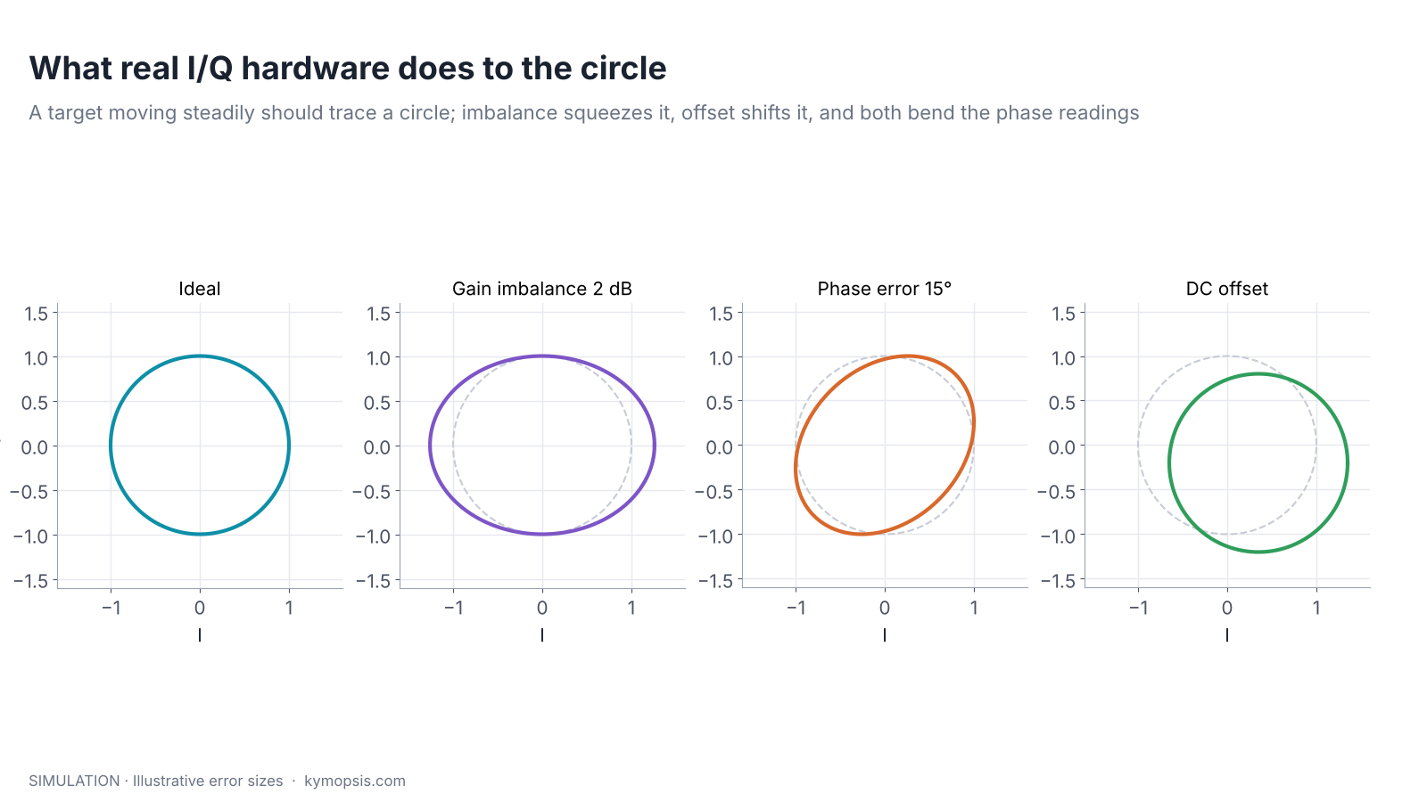
• Gain imbalance: the I and Q paths amplify differently, so the circle becomes an ellipse.
• Phase (quadrature) error: the shift is not exactly 90°, so the ellipse tilts.
• DC offset: leakage from the transmitter, reflections from the radome and static objects add a constant vector, so the circle moves away from the origin.

Each of these makes the phase computed by atan2 run unevenly around the circle. For a gesture detector this hardly matters. For phase ranging and vital-sign sensing, where the motion of interest is a fraction of a millimetre, it shows up directly as a distortion of the measured displacement. The standard correction is to record a few full turns, fit an ellipse to the I/Q points, and map the ellipse back onto a centred circle. Static clutter (the DC part) is removed first, often by subtracting the average over time.

A minimal ellipse correction

Remove the mean of I and Q to cancel the DC offset. Scale Q so that its standard deviation equals that of I to cancel gain imbalance. Then estimate the phase error ε from the correlation of I and Q, sin ε ≈ 2⟨IQ⟩ / (⟨I²⟩ + ⟨Q²⟩), and rebuild Q’ = (Q − I sin ε) / cos ε. This works when the recording covers at least one full turn of phase; for a target that barely moves, use a calibration recording of a moving reflector.

Wrapping and unwrapping

A clock shows 11 and then 1, but it does not tell you whether two hours or fourteen hours have passed. Phase is the same: it only shows where the hand points now. Unwrapping is counting the laps, which works as long as you look often enough that the hand never turns more than half a lap between two looks.

atan2 always answers between −180° and +180°. When the real phase grows past +180°, the reading jumps to −180°: the sawtooth in the first figure. To follow a target over more than half a wavelength, software unwraps the phase: whenever two consecutive readings differ by more than 180°, it adds or subtracts 360° to make the curve continuous.

import numpy as np
lam = 299792458 / 60.5e9                  # wavelength, m
phi = np.angle(iq)                        # wrapped phase, rad (iq = complex samples over time)
disp = np.unwrap(phi) * lam / (4 * np.pi)  # displacement, m

Unwrapping only works if the target moves less than a quarter wavelength (half a phase turn) between two readings; at 60.5 GHz that is 1.24 mm per sample. Faster motion makes the jumps ambiguous. That limit is the same one that sets the maximum unambiguous velocity in chapter 10, and chapter 15 shows the ways around it.

Try it yourself

Every figure here is generated by short Python scripts. The open-source radar-basics-sim library builds complex radar data cubes, so you can change the frequency, move a target by a fraction of a wavelength and watch the phase turn.

On real hardware, phase is available wherever a module exposes complex range-bin data or raw ADC samples. The development kits below do this processing on the module itself, so you work with their outputs (a gesture code or target information, depending on the firmware) rather than with raw phases. Inside that firmware the physics is the same: gesture direction and presence detection both rely on the sign and rate of phase change. If your project needs raw I/Q or ADC samples, say so in the enquiry form below.

Try it yourself: examples/ch02_phase_iq.py in the open-source radar-basics-sim repository runs the core simulation of this chapter; change the assumptions and see what moves.

GitHub · Kymopsis /radar-basics-simView repository → B2B engineering · KymopsisNeed this built into your product?Custom radar modules, antennas and enclosures, from prototype to volume. Send your requirements and we reply with options and a quote.Request a quote →

FAQ

Why does the phase turn once every half wavelength and not every wavelength?

Because the echo travels to the target and back. Moving the target by λ/2 lengthens the round trip by a full λ.

Is Q just I delayed by a quarter period?

For a single steady tone, yes, Q is I shifted by 90°. For a signal that changes (several targets, moving targets, noise) the two channels carry independent information, which is why both are sampled.

Can I measure absolute distance from phase alone?

No. Phase repeats every λ/2, so it only gives distance modulo 2.48 mm at 60 GHz. Radars combine a coarse range from the beat frequency with the fine phase; chapter 9 shows how.

What is the difference between I/Q data and a range-Doppler map?

I/Q samples are the raw complex receiver output over time. A range-Doppler map is computed from them with two FFTs; chapter 10 builds one step by step.

Sources and method

• M. A. Richards, Fundamentals of Radar Signal Processing, 2nd ed., McGraw-Hill, 2014 (complex signal representation, coherent detection).
• M. I. Skolnik, Introduction to Radar Systems, 3rd ed., McGraw-Hill, 2001 (CW and Doppler radar).
• Texas Instruments, Introduction to mmWave Sensing: FMCW Radars, training series, and the mmWave device documentation on real and complex baseband modes (concepts only).
• Figures and animations are computed in Python from the formulas shown; the simulation code is open source in Kymopsis/radar-basics-sim. Figures marked SIMULATION are not measurements of a product.